#THE BIG SHORT
Our motivation of doing this mainly comes from the movie “The Big Short”.
The background of this movie is the well-known subprime mortgage crisis:
The United States subprime mortgage crisis was a multinational financial crisis that occurred between 2007 and 2010 that contributed to the 2007–2008 global financial crisis. It was triggered by a large decline in US home prices after the collapse of a housing bubble, leading to mortgage delinquencies, foreclosures, and the devaluation of housing-related securities. Declines in residential investment preceded the Great Recession and were followed by reductions in household spending and then business investment. Spending reductions were more significant in areas with a combination of high household debt and larger housing price declines.
in 2005, eccentric hedge fund manager Michael Burry discovers that the United States housing market, based on high-risk subprime loans, is extremely unstable. Anticipating the market’s collapse in the second quarter of 2007, as interest rates would rise from adjustable-rate mortgages, he proposes to create a credit default swap market, allowing him to bet against, or short, market-based mortgage-backed securities, for profit.
His long-term bet, exceeding 1 billion, is accepted by major investment and commercial banks but requires paying substantial monthly premiums. This sparks his main client, Lawrence Fields, to accuse him of “wasting” capital while many clients demand that he reverse and sell, but Burry refuses. Under pressure, he eventually restricts withdrawals, angering investors, and Lawrence sues Burry. Eventually, the market collapses and his fund’s value increases by 489% with an overall profit (even allowing for the massive premiums) of over 2.69 billion, with Fields receiving $489 million alone.

The Big Short
#Mortgage-backed Securities
Mortgage-backed Securities is mainly a financial product that loaners integrate their receivables together and pack them into a product for sell. It seems hard to understand, and let’s have an example: Suppose Yusen Wu loaned out 100 bucks to Ke Lan and Ke agreed to pay back 110 bucks one year later, and Yusen also loaned out(lend) 100 bucks to Jackie Xia and he promised to pay back 105 bucks 1 year later, and now Yusen know that he will receive 215 bucks one year later. Now, suppose Yusen Wu sell this ownership of “owing money” to Jianing Yu for 205 bucks, there will be a win-win. Yusen Wu loaned 200 bucks but received 205 bucks immediately, and Jianing Yu know that she will receive 215 bucks one year later for a cost of 205 bucks right now.
Please notice that, receiving the ownership of securities, Jianing can trade again for a different price and earn the profit, and that’s how people use money to generate money.
This is how MBS works. Investment bankings create a market for willing buyers and sellers to trade this kind of securities, but it remains risks: if Ke Lan refuse to pay back the money, Jianing Yu will take the risk.
#Bond Rating To eliminate the risk of default, investment bankings will find rating companies to rate securities by the probability of default. The rating AAA means it is almost surely safe while BBB means not that safe. AAA will have lower interest rates and BBB will have higher, because the higher the risks are, the higher the returns will be.
The delinquicy of rating companies partially caused the subprime mortgage crisis. It was said that almost 95% of bonds were rate AAA while a large portion of them did not have high confidence of payback.
#What Did Big Shorts Find In the movie, those people began to have an idea: short the mortgage security market. They signed deals function as insurance with investment bankings. If the market works fine, they will keep paying the premium to investment companies, but if the market breaks down, the investment company will compensate a huge amount of money. They signed the deal mainly because they are confident that the market will fall down one day.
Why they Believe the market will fall down?
Interest Rates They found out that the interest rate set by loaners were really really low mainly because loaners want to give incentives to people to borrow money, but the low interest rate will attract many borrowers who have no idea whether they can pay back the money
FICO Score The FICO Score is the measure of whether borrowers are reliable, but the investigation of the FICO score was sketchy meaning that many low-FICO score borrowers can borrow the money
LTV ratio The LTV ratio can be understood as the leverage of individual assets. If the LTV ratio is too high there is a high probability that the money will not be paid off.
Discerning three variables, the “shorters” began to believe the market will fall down. This observation also motivates us to do this project. We collected data from 2000 ~ 2014 and want to test whether these variables are strong indicators. Furthermore, we want to see whether other variables will function as strong indicators for one to default.
Finally, we want to do an app that input some number of different variables and it will return the likelihood of default, because we believe loaners must be responsible for figuring out whether they are lending to trustable people. Even though the SEC allows loaners to transit the risks to other people, it does not mean that they can freely lending to anyone else. After the crisis, the government and Central Bank strengthen the censorship of MBS market and banned some financial products like CDO, but we observed that these products still remain in the market with different names, so we must be careful.
## ── Attaching packages ─────────────────────────────────────── tidyverse 1.3.1 ──## ✓ ggplot2 3.3.5 ✓ purrr 0.3.4
## ✓ tibble 3.1.2 ✓ dplyr 1.0.7
## ✓ tidyr 1.1.4 ✓ stringr 1.4.0
## ✓ readr 2.0.1 ✓ forcats 0.5.1## ── Conflicts ────────────────────────────────────────── tidyverse_conflicts() ──
## x dplyr::filter() masks stats::filter()
## x dplyr::lag() masks stats::lag()## Linking to GEOS 3.8.1, GDAL 3.2.1, PROJ 7.2.1## Registered S3 methods overwritten by 'stars':
## method from
## st_bbox.SpatRaster sf
## st_crs.SpatRaster sf## Rows: 619660 Columns: 32## ── Column specification ────────────────────────────────────────────────────────
## Delimiter: ","
## chr (3): state_orig_time, month, day
## dbl (29): id, time, orig_time, first_time, mat_time, res_time, balance_time,...##
## ℹ Use `spec()` to retrieve the full column specification for this data.
## ℹ Specify the column types or set `show_col_types = FALSE` to quiet this message.library(tidyverse)
library(sf)
library(tmap)
library(formattable)
mortgage <-read_csv(here::here('dataset','dcr_clean.csv'))## Rows: 619660 Columns: 32## ── Column specification ────────────────────────────────────────────────────────
## Delimiter: ","
## chr (3): state_orig_time, month, day
## dbl (29): id, time, orig_time, first_time, mat_time, res_time, balance_time,...##
## ℹ Use `spec()` to retrieve the full column specification for this data.
## ℹ Specify the column types or set `show_col_types = FALSE` to quiet this message.mortgage_last<-mortgage %>% group_by(id) %>% summarise_all(last)
epsg_us_equal_area <- 2163
us_states <- st_read(here::here("dataset/cb_2019_us_state_20m/cb_2019_us_state_20m.shp"))%>%
st_transform(epsg_us_equal_area)## Reading layer `cb_2019_us_state_20m' from data source
## `/Users/alex/Desktop/fa2021-final-project-digfora/dataset/cb_2019_us_state_20m/cb_2019_us_state_20m.shp'
## using driver `ESRI Shapefile'
## Simple feature collection with 52 features and 9 fields
## Geometry type: MULTIPOLYGON
## Dimension: XY
## Bounding box: xmin: -179.1743 ymin: 17.91377 xmax: 179.7739 ymax: 71.35256
## Geodetic CRS: NAD83not_contiguous <-
c("Guam", "Commonwealth of the Northern Mariana Islands",
"American Samoa", "Puerto Rico", "Alaska", "Hawaii",
"United States Virgin Islands")
us_cont <- us_states %>%
filter(!NAME %in% not_contiguous) %>% filter(NAME != "District of Columbia") %>%
transmute(STUSPS,STATEFP,NAME, geometry)
p <- mortgage %>% group_by(state_orig_time) %>% summarize(count = n(),def = sum(status_time[status_time == 1])) %>% mutate(proportion = formattable::percent(def / count))
us_cont %>% inner_join(p, by = c("STUSPS" = "state_orig_time")) %>% tm_shape() + tm_polygons(col = "proportion",palette = "RdBu") + tm_text("STUSPS", size = 1/2) + tm_layout(title= 'percentage of number of default')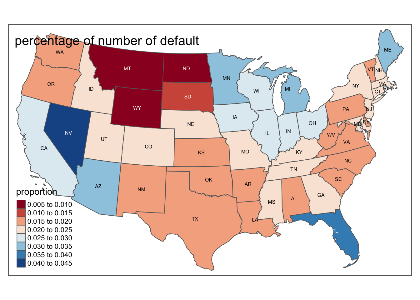
q <- mortgage %>% group_by(state_orig_time) %>% summarize(total = sum(balance_orig_time),def = sum(balance_orig_time[status_time == 1])) %>% mutate(proportion = formattable::percent(def / total))
us_cont %>% inner_join(q, by = c("STUSPS" = "state_orig_time")) %>% tm_shape() + tm_polygons(col = "proportion",palette = "RdBu") +  tm_text("STUSPS", size = 1/2) +  tm_layout(title= 'percentage of default amount')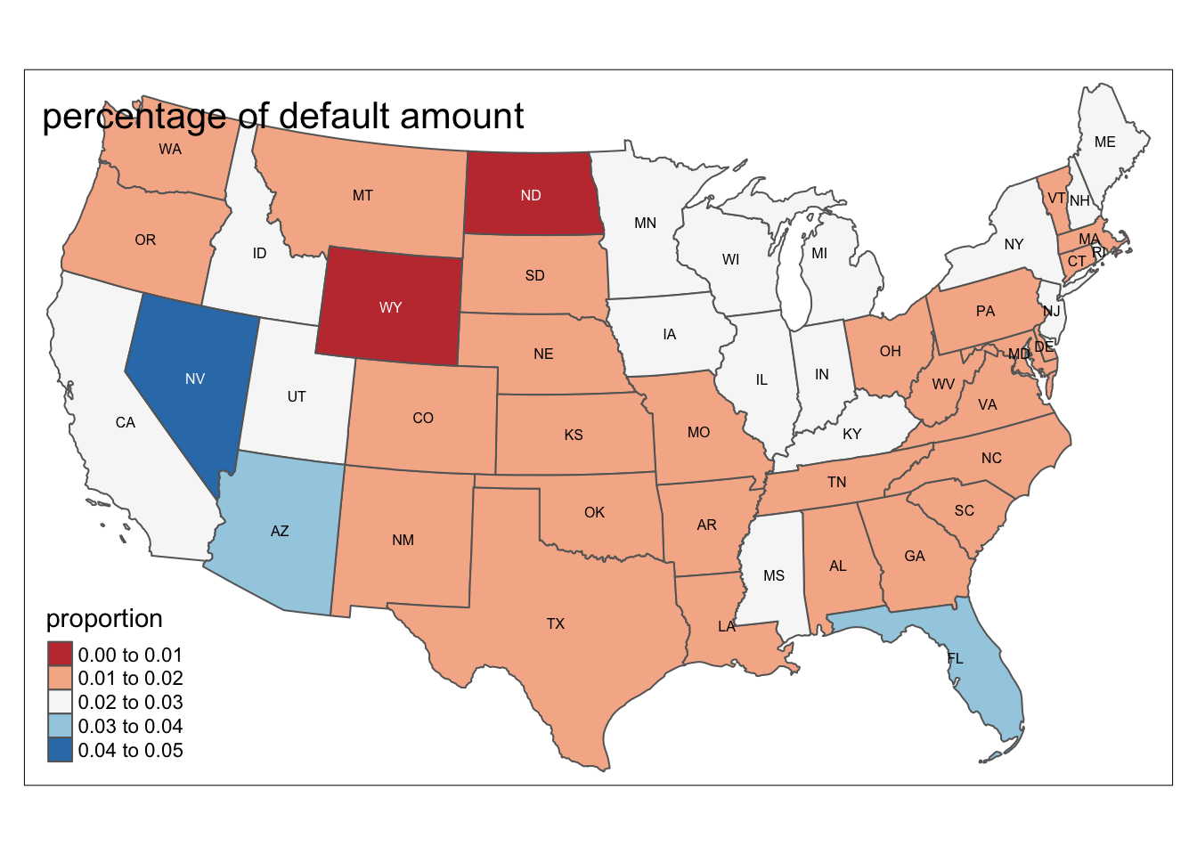
According to this map, we can find out that Montana(MT), Wyoming(WY), North Dakota(ND) have the lowest proportions of default, which are from 0.5 to 1 percent; South Dakota(SD) also has low proportion of default from 1 to 1.5 percents. In contrast, Nevada(NV) has the highest proportion of default, which might caused by the schools with the highest student loan default rates.
We carefully explored multiple variables which are associated with default status, and we will further talk about three of them: mean GDP, mean interest rate, and unemployment rate.
library(modelr)
mor_mod <- glm(default_time ~ gdp_mean, data = mortgage_all, family = binomial)
(beta <- coef(mor_mod))
## (Intercept) gdp_mean
## 0.5131527 -0.8144658library(modelr)
(grid <- mortgage_all %>% data_grid(gdp_mean) %>%
add_predictions(mor_mod, type = "response"))## # A tibble: 1,520 x 2
## gdp_mean pred
## <dbl> <dbl>
## 1 -3.83 0.974
## 2 -3.74 0.972
## 3 -3.67 0.971
## 4 -3.52 0.967
## 5 -3.16 0.956
## 6 -2.82 0.943
## 7 -2.81 0.943
## 8 -2.70 0.938
## 9 -2.58 0.932
## 10 -2.39 0.922
## # … with 1,510 more rowsggplot(mortgage_all, aes(gdp_mean)) + geom_point(aes(y = default_time),alpha = 0.005) +
geom_line(aes(y = pred), data = grid, color = "red", size = 1)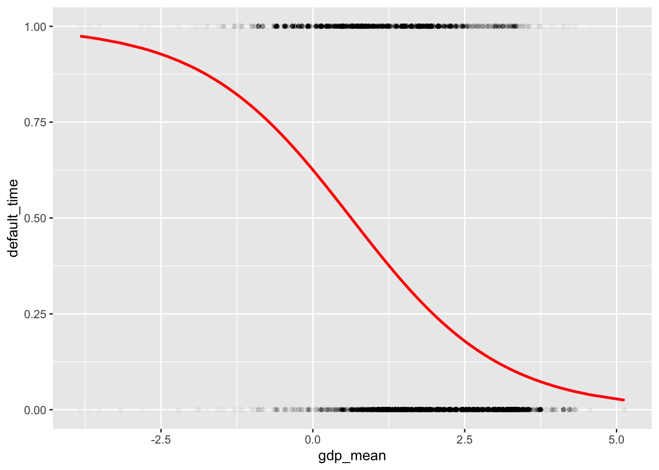 One of the biggest factors that affect default rate is GDP. As we can see from the plot above, when mean GDP increases, the default rate shows a decrease pattern: the higher the GDP, the lower the default rate. This met our expectation because GDP is the most used measure of a country’s standard of living and general economic health. If GDP goes high, meaning citizens’ average living standard is in a high level, and fewer of them will be in a default status.
mor_mod6 <- glm(default_time ~ interest_rate_mean, data = mortgage_all, family = binomial)
(beta <- coef(mor_mod6))
## (Intercept) interest_rate_mean
## -2.6414523 0.2484366library(modelr)
(grid <- mortgage_all %>% data_grid(interest_rate_mean) %>%
add_predictions(mor_mod6, type = "response"))## # A tibble: 10,794 x 2
## interest_rate_mean pred
## <dbl> <dbl>
## 1 0 0.0665
## 2 0.417 0.0732
## 3 1.12 0.0861
## 4 1.38 0.0911
## 5 1.44 0.0924
## 6 1.69 0.0978
## 7 1.72 0.0985
## 8 1.75 0.0992
## 9 1.81 0.101
## 10 1.94 0.103
## # … with 10,784 more rowsggplot(mortgage_all, aes(interest_rate_mean)) + geom_point(aes(y = default_time),alpha = 0.005) +
geom_line(aes(y = pred), data = grid, color = "red", size = 1)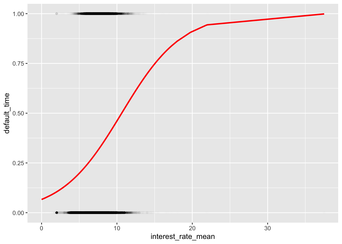 The default rate, also called penalty rate, may refer to the higher interest rate imposed on a borrower who has missed regular payments on a loan. As the above plot shows, the default rate increases dramatically as the average interest rate of all observation periods increases, and default rate tends to be flat from 20 to roughly 37.
mor_mod5 <- glm(default_time ~ uer_mean, data = mortgage_all, family = binomial)
(beta <- coef(mor_mod5))
## (Intercept) uer_mean
## -0.65769799 -0.03024321library(modelr)
(grid <- mortgage_all %>% data_grid(uer_mean) %>%
add_predictions(mor_mod5, type = "response"))## # A tibble: 1,168 x 2
## uer_mean pred
## <dbl> <dbl>
## 1 3.8 0.316
## 2 3.9 0.315
## 3 3.95 0.315
## 4 3.98 0.315
## 5 4 0.315
## 6 4.03 0.314
## 7 4.05 0.314
## 8 4.06 0.314
## 9 4.12 0.314
## 10 4.15 0.314
## # … with 1,158 more rowsggplot(mortgage_all, aes(uer_mean)) + geom_point(aes(y = default_time),alpha = 0.005) +
geom_line(aes(y = pred), data = grid, color = "red", size = 1)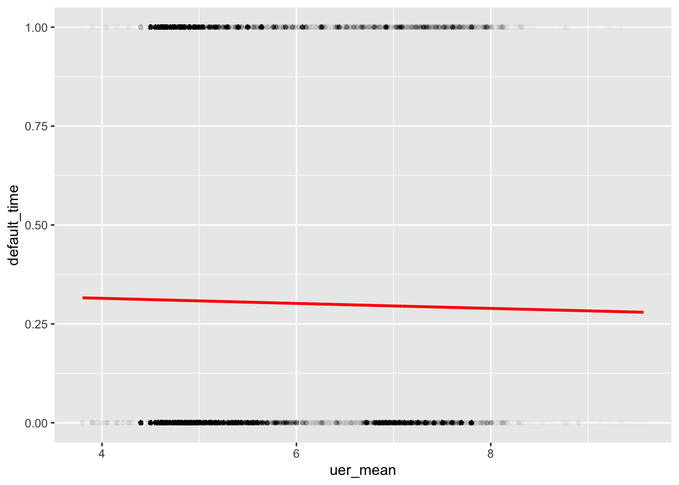 As we can see from the above plot, there is a positive linear relationship between the average unemployment rate and default rate. As the average unemployment rate increases from roughly 4 to 10, the default rate increases from 0.25 to 0.75. This turns out that the increase of unemployment rate lead to higher default rate. Since unemployment means people lost their stable income source, it meets with our expectation to see a higher default rate as unemployment increase.
The bar graph below presents…
Generally speaking, GDP growth, unemployment rate, and the mean interest rate are still the outside dominant factor that may influence one’s default rate. In addition to that, investor house or not,loan to house value ratio, time to maturity are also the inside factor that determines one’s default rate. Therefore, whether one will default or not in a mortgage is strongly related to both the economy of the country and the types of specific mortgage.