This week we use more about model selection and we will add more variables from other datasets to our model
library(tidyverse)## ── Attaching packages ─────────────────────────────────────── tidyverse 1.3.1 ──## ✓ ggplot2 3.3.5 ✓ purrr 0.3.4
## ✓ tibble 3.1.2 ✓ dplyr 1.0.7
## ✓ tidyr 1.1.4 ✓ stringr 1.4.0
## ✓ readr 2.0.1 ✓ forcats 0.5.1## ── Conflicts ────────────────────────────────────────── tidyverse_conflicts() ──
## x dplyr::filter() masks stats::filter()
## x dplyr::lag() masks stats::lag()library(sf)## Linking to GEOS 3.8.1, GDAL 3.2.1, PROJ 7.2.1library(Matrix)##
## Attaching package: 'Matrix'## The following objects are masked from 'package:tidyr':
##
## expand, pack, unpacklibrary(tmap)## Registered S3 methods overwritten by 'stars':
## method from
## st_bbox.SpatRaster sf
## st_crs.SpatRaster sflibrary(formattable)
library(caret)## Loading required package: lattice##
## Attaching package: 'caret'## The following object is masked from 'package:purrr':
##
## liftmortgage <-read_csv(here::here('dataset','dcr_clean.csv'))## Rows: 619660 Columns: 32## ── Column specification ────────────────────────────────────────────────────────
## Delimiter: ","
## chr (3): state_orig_time, month, day
## dbl (29): id, time, orig_time, first_time, mat_time, res_time, balance_time,...##
## ℹ Use `spec()` to retrieve the full column specification for this data.
## ℹ Specify the column types or set `show_col_types = FALSE` to quiet this message.mortgage$age<- mortgage$time-mortgage$orig_time
mortgage$TTM<-mortgage$mat_time-mortgage$orig_time
mortgage$date=paste(as.character(mortgage$year),as.character(mortgage$month),as.character(mortgage$day),sep='-')
mortgage_first<-mortgage[match(unique(mortgage$id), mortgage$id),]
mortgage_first$first_time_date<-mortgage_first$date
mortgage_first$first_time<-mortgage_first$time
first <- mortgage_first %>% select(id, first_time, orig_time,mat_time,rate_time,REtype_CO_orig_time,REtype_PU_orig_time,REtype_SF_orig_time,investor_orig_time,balance_orig_time:Interest_Rate_orig_time,state_orig_time,hpi_orig_time,first_time_date, age, TTM)
get_last <- mortgage %>% select(id,date,time,default_time,payoff_time,status_time) %>% group_by(id) %>% summarise_all(last)
get_last$last_time_date<-get_last$date
get_last$last_time<-get_last$time
get_last$status_last<-get_last$status_time
atlast <- get_last %>% select(id,last_time_date:status_last,default_time)
meanvalue <- mortgage %>% group_by(id) %>% summarise(interest_rate_mean = mean(interest_rate_time),gdp_mean = mean(gdp_time), risk_free_mean = mean(rate_time),hpi_mean = mean(hpi_time),uer_mean = mean(uer_time))
mortgage_all <- first %>% left_join(atlast, by = 'id') %>% left_join(meanvalue, by = 'id')
mortgage_all$time_to_GFC <- 37-mortgage_all$first_time## to increase the accuracy, I use Lasso regression with machine learning
mortgage_ml <- na.omit(mortgage_all)
set.seed(123)
training.samples <- mortgage_ml$default_time %>%
createDataPartition(p = 0.8, list = FALSE)
train.data <- mortgage_ml[training.samples, ]
test.data <- mortgage_ml[-training.samples, ]library(glmnet) ## Loaded glmnet 4.1-3library(faraway)##
## Attaching package: 'faraway'## The following object is masked from 'package:lattice':
##
## melanomax <- model.matrix(default_time ~ age + TTM+ last_time+ status_last+ interest_rate_mean+gdp_mean*uer_mean+ risk_free_mean+ hpi_mean+ FICO_orig_time+ hpi_mean,
data = train.data)[,-1]
y <- ifelse(train.data$default_time == 1, 1, 0)
glmnet(x, y, family = "binomial", alpha = 1, lambda = NULL)##
## Call: glmnet(x = x, y = y, family = "binomial", alpha = 1, lambda = NULL)
##
## Df %Dev Lambda
## 1 0 0.00 0.194000
## 2 1 2.45 0.176800
## 3 1 4.47 0.161100
## 4 1 6.15 0.146700
## 5 2 7.58 0.133700
## 6 2 9.59 0.121800
## 7 2 11.30 0.111000
## 8 2 12.76 0.101100
## 9 2 14.00 0.092160
## 10 3 15.51 0.083970
## 11 3 17.01 0.076510
## 12 4 20.71 0.069720
## 13 4 24.04 0.063520
## 14 4 26.98 0.057880
## 15 4 29.58 0.052740
## 16 4 31.90 0.048050
## 17 4 33.96 0.043780
## 18 5 35.98 0.039890
## 19 5 37.88 0.036350
## 20 5 39.58 0.033120
## 21 6 41.09 0.030180
## 22 6 42.47 0.027500
## 23 7 43.71 0.025050
## 24 8 44.82 0.022830
## 25 8 45.81 0.020800
## 26 8 46.68 0.018950
## 27 8 47.45 0.017270
## 28 8 48.11 0.015740
## 29 8 48.70 0.014340
## 30 10 49.26 0.013060
## 31 10 50.15 0.011900
## 32 10 50.97 0.010850
## 33 11 51.72 0.009882
## 34 11 52.66 0.009004
## 35 10 53.45 0.008204
## 36 10 54.07 0.007475
## 37 10 54.62 0.006811
## 38 10 55.11 0.006206
## 39 10 55.54 0.005655
## 40 10 55.92 0.005153
## 41 10 56.24 0.004695
## 42 10 56.53 0.004278
## 43 10 56.78 0.003898
## 44 10 57.00 0.003551
## 45 10 57.18 0.003236
## 46 10 57.35 0.002948
## 47 10 57.49 0.002687
## 48 10 57.61 0.002448
## 49 10 57.71 0.002230
## 50 10 57.80 0.002032
## 51 10 57.88 0.001852
## 52 10 57.94 0.001687
## 53 10 58.00 0.001537
## 54 10 58.05 0.001401
## 55 10 58.09 0.001276
## 56 11 58.15 0.001163
## 57 11 58.37 0.001060
## 58 11 58.55 0.000966
## 59 11 58.71 0.000880
## 60 11 58.84 0.000802
## 61 11 58.95 0.000730
## 62 11 59.04 0.000665
## 63 11 59.11 0.000606
## 64 11 59.17 0.000553
## 65 11 59.23 0.000503
## 66 11 59.27 0.000459
## 67 11 59.31 0.000418
## 68 11 59.34 0.000381
## 69 11 59.36 0.000347
## 70 11 59.38 0.000316
## 71 11 59.40 0.000288
## 72 11 59.42 0.000262
## 73 11 59.43 0.000239
## 74 11 59.44 0.000218
## 75 11 59.45 0.000199
## 76 11 59.46 0.000181
## 77 11 59.46 0.000165
## 78 11 59.47 0.000150
## 79 11 59.47 0.000137
## 80 11 59.48 0.000125
## 81 11 59.48 0.000114
## 82 11 59.48 0.000104
## 83 11 59.48 0.000094
## 84 11 59.48 0.000086
## 85 11 59.49 0.000078
## 86 11 59.49 0.000071set.seed(123)
cv.lasso <- cv.glmnet(x, y, alpha = 1, family = "binomial")
model <- glmnet(x, y, alpha = 1, family = "binomial",
lambda = cv.lasso$lambda.min)
coef(model)## 12 x 1 sparse Matrix of class "dgCMatrix"
## s0
## (Intercept) -4.576481886
## age -0.041744705
## TTM 0.021109214
## last_time -0.444417226
## status_last -5.352373253
## interest_rate_mean 0.075824269
## gdp_mean -7.199292425
## uer_mean 1.662571752
## risk_free_mean -0.357088532
## hpi_mean 0.117828076
## FICO_orig_time -0.003016795
## gdp_mean:uer_mean 0.774048073x.test <- model.matrix(default_time ~ age + TTM+ last_time+ status_last+ interest_rate_mean+gdp_mean*uer_mean+ risk_free_mean+ hpi_mean+ FICO_orig_time+ hpi_mean, test.data)[,-1]
probabilities <- model %>% predict(newx = x.test)
predicted.classes <- ifelse(probabilities > 0.5, "default", "payback")
library(glmnet)
set.seed(123)
cv.lasso <- cv.glmnet(x, y, alpha = 1, family = "binomial")
plot(cv.lasso)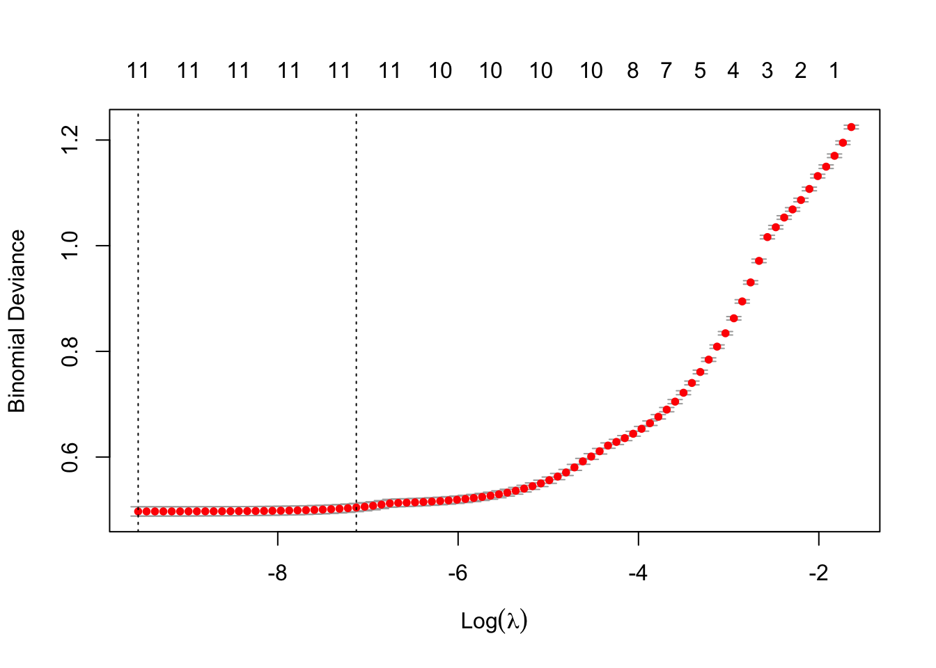
cv.lasso$lambda.min## [1] 7.135674e-05cv.lasso$lambda.1se## [1] 0.0008015674coef(cv.lasso, cv.lasso$lambda.min)## 12 x 1 sparse Matrix of class "dgCMatrix"
## s1
## (Intercept) -4.538261067
## age -0.041706498
## TTM 0.021097993
## last_time -0.443585296
## status_last -5.346884481
## interest_rate_mean 0.075829728
## gdp_mean -7.170121997
## uer_mean 1.658933176
## risk_free_mean -0.357121952
## hpi_mean 0.117502011
## FICO_orig_time -0.003014254
## gdp_mean:uer_mean 0.769563666##Using lambda.1se as the best lambda, gives the following regression coefficients:
coef(cv.lasso, cv.lasso$lambda.1se)## 12 x 1 sparse Matrix of class "dgCMatrix"
## s1
## (Intercept) -1.774807825
## age -0.035866922
## TTM 0.019528984
## last_time -0.372909642
## status_last -4.943609179
## interest_rate_mean 0.067435512
## gdp_mean -4.050056636
## uer_mean 1.474202368
## risk_free_mean -0.352693658
## hpi_mean 0.089116206
## FICO_orig_time -0.002741908
## gdp_mean:uer_mean 0.272358675# Final model with lambda.min
lasso.model <- glmnet(x, y, alpha = 1, family = "binomial",
lambda = cv.lasso$lambda.min)
# Make prediction on test data
x.test <- model.matrix(default_time ~ age + TTM+ last_time+ status_last+ interest_rate_mean+gdp_mean*uer_mean+ risk_free_mean+ hpi_mean+ FICO_orig_time+ hpi_mean, test.data)[,-1]
probabilities <- lasso.model %>% predict(newx = x.test)
predicted.classes <- ifelse(probabilities > 0.5, 1, 0)
# Model accuracy
observed.classes <- test.data$default_time
mean(predicted.classes == observed.classes)## [1] 0.9334605# Final model with lambda.1se
lasso.model <- glmnet(x, y, alpha = 1, family = "binomial",
lambda = cv.lasso$lambda.1se)
# Make prediction on test data
x.test <- model.matrix(default_time ~ age + TTM+ last_time+ status_last+ interest_rate_mean+gdp_mean*uer_mean+ risk_free_mean+ hpi_mean+ FICO_orig_time+ hpi_mean, test.data)[,-1]
probabilities <- lasso.model %>% predict(newx = x.test)
predicted.classes <- ifelse(probabilities > 0.5, 1, 0)
# Model accuracy rate
observed.classes <- test.data$default_time
mean(predicted.classes == observed.classes)## [1] 0.9356684# Fit the model
full.model <- glm(default_time ~ age + TTM+ last_time+ status_last+ interest_rate_mean+gdp_mean*uer_mean+ risk_free_mean+ hpi_mean+ FICO_orig_time+ hpi_mean, data = train.data, family = binomial)
# Make predictions
probabilities <- full.model %>% predict(test.data, type = "response")
predicted.classes <- ifelse(probabilities > 0.5, 1, 0)
# Model accuracy
observed.classes <- test.data$default_time
mean(predicted.classes == observed.classes)## [1] 0.9420915library(modelr)
library(pROC)## Type 'citation("pROC")' for a citation.##
## Attaching package: 'pROC'## The following objects are masked from 'package:stats':
##
## cov, smooth, varfull.model##
## Call: glm(formula = default_time ~ age + TTM + last_time + status_last +
## interest_rate_mean + gdp_mean * uer_mean + risk_free_mean +
## hpi_mean + FICO_orig_time + hpi_mean, family = binomial,
## data = train.data)
##
## Coefficients:
## (Intercept) age TTM last_time
## -5.012578 -0.042306 0.021325 -0.454664
## status_last interest_rate_mean gdp_mean uer_mean
## -5.415270 0.076664 -7.604302 1.698916
## risk_free_mean hpi_mean FICO_orig_time gdp_mean:uer_mean
## -0.360264 0.121955 -0.003055 0.836962
##
## Degrees of Freedom: 39855 Total (i.e. Null); 39844 Residual
## Null Deviance: 48820
## Residual Deviance: 19770 AIC: 19800mortgage_all <- mortgage_all %>% add_predictions(full.model, type = 'response')
roc(mortgage_all$default_time,mortgage_all$pred,plot = TRUE)## Setting levels: control = 0, case = 1## Setting direction: controls < cases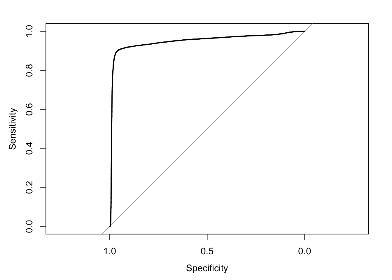
##
## Call:
## roc.default(response = mortgage_all$default_time, predictor = mortgage_all$pred,     plot = TRUE)
##
## Data: mortgage_all$pred in 34703 controls (mortgage_all$default_time 0) < 15117 cases (mortgage_all$default_time 1).
## Area under the curve: 0.949