The map in last blog post is a little hard to make too much sense of since it largely just reflects population, so we revised it.
library(tidyverse)## ── Attaching packages ─────────────────────────────────────── tidyverse 1.3.1 ──## ✓ ggplot2 3.3.5 ✓ purrr 0.3.4
## ✓ tibble 3.1.2 ✓ dplyr 1.0.7
## ✓ tidyr 1.1.4 ✓ stringr 1.4.0
## ✓ readr 2.0.1 ✓ forcats 0.5.1## ── Conflicts ────────────────────────────────────────── tidyverse_conflicts() ──
## x dplyr::filter() masks stats::filter()
## x dplyr::lag() masks stats::lag()library(sf)## Linking to GEOS 3.8.1, GDAL 3.2.1, PROJ 7.2.1library(tmap)## Registered S3 methods overwritten by 'stars':
## method from
## st_bbox.SpatRaster sf
## st_crs.SpatRaster sflibrary(formattable)
mortgage <-read_csv(here::here('dataset','dcr_clean.csv'))## Rows: 619660 Columns: 32## ── Column specification ────────────────────────────────────────────────────────
## Delimiter: ","
## chr (3): state_orig_time, month, day
## dbl (29): id, time, orig_time, first_time, mat_time, res_time, balance_time,...##
## ℹ Use `spec()` to retrieve the full column specification for this data.
## ℹ Specify the column types or set `show_col_types = FALSE` to quiet this message.mortgage_last<-mortgage %>% group_by(id) %>% summarise_all(last)
epsg_us_equal_area <- 2163
us_states <- st_read(here::here("dataset/cb_2019_us_state_20m/cb_2019_us_state_20m.shp"))%>%
st_transform(epsg_us_equal_area)## Reading layer `cb_2019_us_state_20m' from data source
## `/Users/alex/Desktop/fa2021-final-project-digfora/dataset/cb_2019_us_state_20m/cb_2019_us_state_20m.shp'
## using driver `ESRI Shapefile'
## Simple feature collection with 52 features and 9 fields
## Geometry type: MULTIPOLYGON
## Dimension: XY
## Bounding box: xmin: -179.1743 ymin: 17.91377 xmax: 179.7739 ymax: 71.35256
## Geodetic CRS: NAD83not_contiguous <-
c("Guam", "Commonwealth of the Northern Mariana Islands",
"American Samoa", "Puerto Rico", "Alaska", "Hawaii",
"United States Virgin Islands")
us_cont <- us_states %>%
filter(!NAME %in% not_contiguous) %>% filter(NAME != "District of Columbia") %>%
transmute(STUSPS,STATEFP,NAME, geometry)
p <- mortgage %>% group_by(state_orig_time) %>% summarize(count = n(),def = sum(status_time[status_time == 1])) %>% mutate(proportion = formattable::percent(def / count))
us_cont %>% inner_join(p, by = c("STUSPS" = "state_orig_time")) %>% tm_shape() + tm_polygons(col = "proportion",palette = "RdBu") + tm_text("STUSPS", size = 1/2) + tm_layout(title= 'percentage of number of default')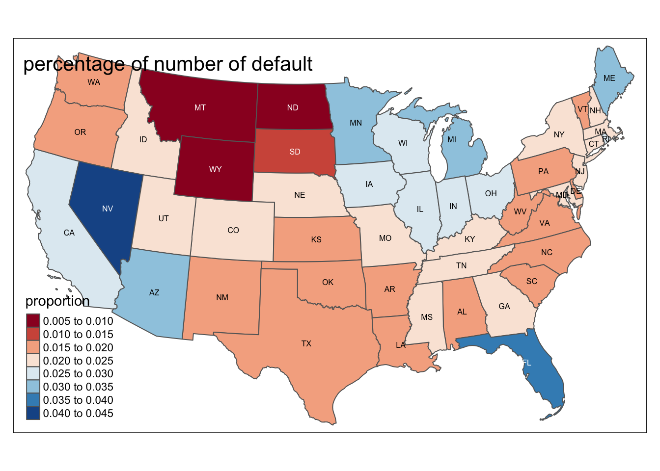
q <- mortgage %>% group_by(state_orig_time) %>% summarize(total = sum(balance_orig_time),def = sum(balance_orig_time[status_time == 1])) %>% mutate(proportion = formattable::percent(def / total))
us_cont %>% inner_join(q, by = c("STUSPS" = "state_orig_time")) %>% tm_shape() + tm_polygons(col = "proportion",palette = "RdBu") +  tm_text("STUSPS", size = 1/2) +  tm_layout(title= 'percentage of default amount')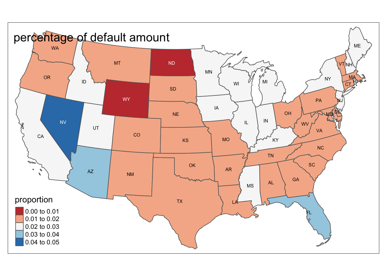
For this week, we are starting a construct a model to predict default rate of certain mortgage. Since we have a panel dataset–multiple records refer to a same mortgage over different period. We would not know whether a mortgage is default or payoff until we see last record of this mortgage. Therefore, it is a little bit complicated for us to build a logistic linear regression. We then decided to normalized the dataset again and try to collapse them to build a dataset with have only one record for one mortgage, including their start time, end time, their age,avergae GDP during the mortgage, status at last(default or pay off) and etc.
Firstly, we would like to determine the start time, age, time to maturity of We start by loading the dataset and packages:
library(tidyverse)
mortgage <- read_csv(here::here('dataset','dcr_clean.csv'))
## Rows: 619660 Columns: 32## ── Column specification ────────────────────────────────────────────────────────
## Delimiter: ","
## chr (3): state_orig_time, month, day
## dbl (29): id, time, orig_time, first_time, mat_time, res_time, balance_time,...##
## ℹ Use `spec()` to retrieve the full column specification for this data.
## ℹ Specify the column types or set `show_col_types = FALSE` to quiet this message.#create a new column for the age of a mortgage
mortgage$age<- mortgage$time-mortgage$orig_time
#create a new column for the time to maturity of a mortgage
mortgage$TTM<-mortgage$mat_time-mortgage$orig_time
#create a continuous time variable for each records
mortgage$date=paste(as.character(mortgage$year),as.character(mortgage$month),as.character(mortgage$day),sep='-')
#found out the first-time record for all mortgages
mortgage_first<-mortgage[match(unique(mortgage$id), mortgage$id),]
#create a column for start time of each mortgage
mortgage_first$first_time_date<-mortgage_first$date
mortgage_first$first_time<-mortgage_first$time
#leave only the collumn that contains first time data of the mortgage
first <- mortgage_first %>% select(id, first_time, orig_time,mat_time,rate_time,REtype_CO_orig_time,REtype_PU_orig_time,REtype_SF_orig_time,investor_orig_time,balance_orig_time:Interest_Rate_orig_time,state_orig_time,hpi_orig_time,first_time_date, age, TTM)As followed, we would like to determine the ending status of each mortgage(defualt, pay off or unfnished):
#Get the last record for all mortgages in the dataset
get_last <- mortgage %>% select(id,date,time,default_time,payoff_time,status_time) %>% group_by(id) %>% summarise_all(last)
#determine the end time of a mortgage
get_last$last_time_date<-get_last$date
get_last$last_time<-get_last$time
#determine the status of the mortgage
get_last$status_last<-get_last$status_time
atlast <- get_last %>% select(id,last_time_date:status_last,default_time)
As followed, we would like to get the mean value of GDP growth, Unemployment Rate, Risk_free rate, interest rate, house price index for each mortgage from their start to their end.
meanvalue <- mortgage %>% group_by(id) %>% summarise(interest_rate_mean = mean(interest_rate_time),gdp_mean = mean(gdp_time), risk_free_mean = mean(rate_time),hpi_mean = mean(hpi_time),uer_mean = mean(uer_time))Now We would like to join the three dataset together to form the new dataset with one record for one mortgage:
mortgage_all <- first %>% left_join(atlast, by = 'id') %>% left_join(meanvalue, by = 'id')We would like to add one more variable, time between the start of the mortgage and global financial crisis(time 37) to measure the influence of Financial Crisis to the mortgage
mortgage_all$time_to_GFC <- 37-mortgage_all$first_timeHere is the column expalnation of our new datasets.
newstr<-'id:borrower id
first_time:time stamp for first observation
orig_time:time stamp for origination
mat_time:time stamp for maturity
rate_time:risk-free rate
REtype_CO_orig_time:real estate type condominium: 1, otherwise: 0
REtype_PU_orig_time:real estate type planned urban developments: 1, otherwise: 0
REtype_SF_orig_time:single family home: 1, otherwise: 0
investor_orig_time:investor borrower: 1, otherwise: 0
balance_orig_time:outstanding balance at origination time
FICO_orig_time:FICO score at origination time, in %
LTV_orig_time:loan to value ratio at origination time, in %
Interest_Rate_orig_time:interest rate at origination time, in %
state_orig_time:US state in which the property is located
hpi_orig_time:house price index at observation time, base year=100
first_time_date:date of the first observation
age:number of periods from origination to time of observation
TTM:time to maturity at the time of observation
last_time_date:date of the last observation
last_time:time stamp for the last observation
status_last:debt status at the last observation: 0 is unfinished, 1 is default, 2 is paidoff
interest_rate_mean:the average interest rate of all observation periods
gdp_mean:the average GDP growth of all observation periods
risk_free_mean:the average risk free rate of all observation periods
hpi_mean:the average house price index of all observation periods
uer_mean:the average unemployment rate of all observation periods
time_to_GFC:number of periods from first observation to global financial crisis'

lista<-str_split(newstr, "\n")
keydataname<-data.frame(lista)
colnames(keydataname)<-'dataname'
keydataname<-keydataname %>% separate(dataname,into=c('Column Name','Description'),sep=':')
## Warning: Expected 2 pieces. Additional pieces discarded in 5 rows [6, 7, 8, 9,
## 21].as.tibble(keydataname) %>%knitr::kable()## Warning: `as.tibble()` was deprecated in tibble 2.0.0.
## Please use `as_tibble()` instead.
## The signature and semantics have changed, see `?as_tibble`.| Column Name | Description |
|---|---|
| id | borrower id |
| first_time | time stamp for first observation |
| orig_time | time stamp for origination |
| mat_time | time stamp for maturity |
| rate_time | risk-free rate |
| REtype_CO_orig_time | real estate type condominium |
| REtype_PU_orig_time | real estate type planned urban developments |
| REtype_SF_orig_time | single family home |
| investor_orig_time | investor borrower |
| balance_orig_time | outstanding balance at origination time |
| FICO_orig_time | FICO score at origination time, in % |
| LTV_orig_time | loan to value ratio at origination time, in % |
| Interest_Rate_orig_time | interest rate at origination time, in % |
| state_orig_time | US state in which the property is located |
| hpi_orig_time | house price index at observation time, base year=100 |
| first_time_date | date of the first observation |
| age | number of periods from origination to time of observation |
| TTM | time to maturity at the time of observation |
| last_time_date | date of the last observation |
| last_time | time stamp for the last observation |
| status_last | debt status at the last observation |
| interest_rate_mean | the average interest rate of all observation periods |
| gdp_mean | the average GDP growth of all observation periods |
| risk_free_mean | the average risk free rate of all observation periods |
| hpi_mean | the average house price index of all observation periods |
| uer_mean | the average unemployment rate of all observation periods |
| time_to_GFC | number of periods from first observation to global financial crisis |
Now, we will need to filter out mortgages that are unfinished.
mortgage_all <- mortgage_all %>% filter(status_last != 0)Some of the columns that are not included will be discussed in the future.Now, with the new collapsed dataset, we can start constructing our model. Firstly, we would like to construct a correlation table to determine which varible to be included in our regression fuction.
variable_subset <- mortgage_all[c('first_time','orig_time','mat_time','rate_time','REtype_CO_orig_time','REtype_PU_orig_time','REtype_SF_orig_time','investor_orig_time','balance_orig_time','FICO_orig_time','LTV_orig_time','Interest_Rate_orig_time','hpi_orig_time','age','TTM','last_time','default_time','interest_rate_mean','gdp_mean','risk_free_mean','hpi_mean','uer_mean','time_to_GFC')]

cor(variable_subset) %>% knitr::kable()| first_time | orig_time | mat_time | rate_time | REtype_CO_orig_time | REtype_PU_orig_time | REtype_SF_orig_time | investor_orig_time | balance_orig_time | FICO_orig_time | LTV_orig_time | Interest_Rate_orig_time | hpi_orig_time | age | TTM | last_time | default_time | interest_rate_mean | gdp_mean | risk_free_mean | hpi_mean | uer_mean | time_to_GFC | |
|---|---|---|---|---|---|---|---|---|---|---|---|---|---|---|---|---|---|---|---|---|---|---|---|
| first_time | 1.0000000 | 0.7204394 | 0.4121585 | 0.1138200 | 0.0292483 | 0.0229569 | -0.0307036 | 0.0116296 | 0.1546413 | 0.0824204 | 0.0092745 | 0.0687341 | 0.6929031 | 0.2299836 | 0.1156180 | 0.6148660 | 0.3039482 | -0.1023105 | -0.5424740 | 0.1136880 | 0.1369459 | 0.2936127 | -1.0000000 |
| orig_time | 0.7204394 | 1.0000000 | 0.5918757 | -0.0615906 | 0.0407945 | 0.0610640 | -0.0599190 | 0.0432014 | 0.2098406 | 0.1553459 | -0.0164785 | 0.0160576 | 0.9160574 | -0.5092385 | 0.1846039 | 0.4593792 | 0.2978776 | -0.1435913 | -0.4828428 | -0.0616145 | 0.1433444 | 0.1679640 | -0.7204394 |
| mat_time | 0.4121585 | 0.5918757 | 1.0000000 | -0.0149594 | 0.0350942 | 0.0605812 | -0.0418815 | -0.0198346 | 0.1676437 | 0.0631609 | 0.0632089 | -0.1081868 | 0.5743841 | -0.3190921 | 0.9014386 | 0.2064687 | 0.2295032 | -0.1050570 | -0.2702708 | -0.0153298 | 0.1000367 | 0.0480902 | -0.4121585 |
| rate_time | 0.1138200 | -0.0615906 | -0.0149594 | 1.0000000 | 0.0064903 | -0.0117604 | 0.0253148 | 0.0114580 | -0.0313978 | -0.0780419 | 0.0118861 | 0.1827828 | 0.1063109 | 0.2276740 | 0.0148391 | 0.0809171 | 0.1885953 | 0.2813221 | -0.3139753 | 0.9996952 | -0.1837950 | 0.0154899 | -0.1138200 |
| REtype_CO_orig_time | 0.0292483 | 0.0407945 | 0.0350942 | 0.0064903 | 1.0000000 | -0.0965647 | -0.3415917 | 0.0207958 | -0.0089662 | 0.0915365 | 0.0098910 | -0.0238453 | 0.0521295 | -0.0209500 | 0.0208812 | 0.0322690 | 0.0054182 | -0.0650387 | -0.0295951 | 0.0063323 | 0.0047353 | 0.0114768 | -0.0292483 |
| REtype_PU_orig_time | 0.0229569 | 0.0610640 | 0.0605812 | -0.0117604 | -0.0965647 | 1.0000000 | -0.4690949 | -0.0166762 | 0.0958164 | 0.1242780 | -0.0048864 | -0.0248709 | 0.0658115 | -0.0572009 | 0.0410717 | 0.0454316 | 0.0126085 | -0.1162657 | -0.0339186 | -0.0115687 | 0.0031630 | 0.0253864 | -0.0229569 |
| REtype_SF_orig_time | -0.0307036 | -0.0599190 | -0.0418815 | 0.0253148 | -0.3415917 | -0.4690949 | 1.0000000 | -0.1013132 | -0.0462944 | -0.1319948 | 0.0041750 | -0.0137843 | -0.0682895 | 0.0459809 | -0.0188856 | -0.0405454 | -0.0039875 | 0.0730690 | 0.0052115 | 0.0252423 | -0.0541469 | -0.0119068 | 0.0307036 |
| investor_orig_time | 0.0116296 | 0.0432014 | -0.0198346 | 0.0114580 | 0.0207958 | -0.0166762 | -0.1013132 | 1.0000000 | -0.1168575 | 0.1699794 | -0.0639457 | 0.0956060 | 0.0435371 | -0.0461916 | -0.0473878 | 0.0412416 | 0.0339573 | 0.0340316 | -0.0332389 | 0.0114132 | -0.0052367 | 0.0242550 | -0.0116296 |
| balance_orig_time | 0.1546413 | 0.2098406 | 0.1676437 | -0.0313978 | -0.0089662 | 0.0958164 | -0.0462944 | -0.1168575 | 1.0000000 | 0.3229090 | -0.1935153 | -0.0835764 | 0.1884202 | -0.1025605 | 0.0917100 | 0.1515442 | -0.0010766 | -0.3375744 | -0.1397382 | -0.0314263 | -0.0176242 | 0.1100034 | -0.1546413 |
| FICO_orig_time | 0.0824204 | 0.1553459 | 0.0631609 | -0.0780419 | 0.0915365 | 0.1242780 | -0.1319948 | 0.1699794 | 0.3229090 | 1.0000000 | -0.0995956 | -0.0710463 | 0.1558017 | -0.1157125 | -0.0064203 | 0.2040493 | -0.1082498 | -0.5259041 | -0.1282160 | -0.0777834 | -0.0048778 | 0.1430426 | -0.0824204 |
| LTV_orig_time | 0.0092745 | -0.0164785 | 0.0632089 | 0.0118861 | 0.0098910 | -0.0048864 | 0.0041750 | -0.0639457 | -0.1935153 | -0.0995956 | 1.0000000 | -0.0021603 | -0.0174270 | 0.0346331 | 0.0859226 | -0.0590717 | 0.0888124 | 0.2030012 | 0.0499672 | 0.0119659 | 0.0528514 | -0.0554563 | -0.0092745 |
| Interest_Rate_orig_time | 0.0687341 | 0.0160576 | -0.1081868 | 0.1827828 | -0.0238453 | -0.0248709 | -0.0137843 | 0.0956060 | -0.0835764 | -0.0710463 | -0.0021603 | 1.0000000 | 0.0467439 | 0.0627628 | -0.1405393 | 0.0873160 | 0.1052690 | 0.2503181 | -0.1808460 | 0.1828129 | -0.1402862 | 0.0448506 | -0.0687341 |
| hpi_orig_time | 0.6929031 | 0.9160574 | 0.5743841 | 0.1063109 | 0.0521295 | 0.0658115 | -0.0682895 | 0.0435371 | 0.1884202 | 0.1558017 | -0.0174270 | 0.0467439 | 1.0000000 | -0.4256156 | 0.2083603 | 0.4535288 | 0.3074560 | -0.1397604 | -0.4880450 | 0.1062585 | 0.2426822 | 0.0863770 | -0.6929031 |
| age | 0.2299836 | -0.5092385 | -0.3190921 | 0.2276740 | -0.0209500 | -0.0572009 | 0.0459809 | -0.0461916 | -0.1025605 | -0.1157125 | 0.0346331 | 0.0627628 | -0.4256156 | 1.0000000 | -0.1155728 | 0.1183877 | -0.0408169 | 0.0745348 | 0.0043735 | 0.2275439 | -0.0312074 | 0.1286613 | -0.2299836 |
| TTM | 0.1156180 | 0.1846039 | 0.9014386 | 0.0148391 | 0.0208812 | 0.0410717 | -0.0188856 | -0.0473878 | 0.0917100 | -0.0064203 | 0.0859226 | -0.1405393 | 0.2083603 | -0.1155728 | 1.0000000 | 0.0050268 | 0.1198535 | -0.0509779 | -0.0702203 | 0.0144003 | 0.0449892 | -0.0315734 | -0.1156180 |
| last_time | 0.6148660 | 0.4593792 | 0.2064687 | 0.0809171 | 0.0322690 | 0.0454316 | -0.0405454 | 0.0412416 | 0.1515442 | 0.2040493 | -0.0590717 | 0.0873160 | 0.4535288 | 0.1183877 | 0.0050268 | 1.0000000 | 0.2975575 | -0.2200291 | -0.6949821 | 0.0814640 | -0.2450211 | 0.7209687 | -0.6148660 |
| default_time | 0.3039482 | 0.2978776 | 0.2295032 | 0.1885953 | 0.0054182 | 0.0126085 | -0.0039875 | 0.0339573 | -0.0010766 | -0.1082498 | 0.0888124 | 0.1052690 | 0.3074560 | -0.0408169 | 0.1198535 | 0.2975575 | 1.0000000 | 0.1516563 | -0.4493496 | 0.1884337 | -0.1671072 | 0.1808916 | -0.3039482 |
| interest_rate_mean | -0.1023105 | -0.1435913 | -0.1050570 | 0.2813221 | -0.0650387 | -0.1162657 | 0.0730690 | 0.0340316 | -0.3375744 | -0.5259041 | 0.2030012 | 0.2503181 | -0.1397604 | 0.0745348 | -0.0509779 | -0.2200291 | 0.1516563 | 1.0000000 | -0.0229672 | 0.2810567 | -0.1204072 | -0.1729804 | 0.1023105 |
| gdp_mean | -0.5424740 | -0.4828428 | -0.2702708 | -0.3139753 | -0.0295951 | -0.0339186 | 0.0052115 | -0.0332389 | -0.1397382 | -0.1282160 | 0.0499672 | -0.1808460 | -0.4880450 | 0.0043735 | -0.0702203 | -0.6949821 | -0.4493496 | -0.0229672 | 1.0000000 | -0.3140921 | 0.4424599 | -0.5565366 | 0.5424740 |
| risk_free_mean | 0.1136880 | -0.0616145 | -0.0153298 | 0.9996952 | 0.0063323 | -0.0115687 | 0.0252423 | 0.0114132 | -0.0314263 | -0.0777834 | 0.0119659 | 0.1828129 | 0.1062585 | 0.2275439 | 0.0144003 | 0.0814640 | 0.1884337 | 0.2810567 | -0.3140921 | 1.0000000 | -0.1840000 | 0.0159213 | -0.1136880 |
| hpi_mean | 0.1369459 | 0.1433444 | 0.1000367 | -0.1837950 | 0.0047353 | 0.0031630 | -0.0541469 | -0.0052367 | -0.0176242 | -0.0048778 | 0.0528514 | -0.1402862 | 0.2426822 | -0.0312074 | 0.0449892 | -0.2450211 | -0.1671072 | -0.1204072 | 0.4424599 | -0.1840000 | 1.0000000 | -0.6671533 | -0.1369459 |
| uer_mean | 0.2936127 | 0.1679640 | 0.0480902 | 0.0154899 | 0.0114768 | 0.0253864 | -0.0119068 | 0.0242550 | 0.1100034 | 0.1430426 | -0.0554563 | 0.0448506 | 0.0863770 | 0.1286613 | -0.0315734 | 0.7209687 | 0.1808916 | -0.1729804 | -0.5565366 | 0.0159213 | -0.6671533 | 1.0000000 | -0.2936127 |
| time_to_GFC | -1.0000000 | -0.7204394 | -0.4121585 | -0.1138200 | -0.0292483 | -0.0229569 | 0.0307036 | -0.0116296 | -0.1546413 | -0.0824204 | -0.0092745 | -0.0687341 | -0.6929031 | -0.2299836 | -0.1156180 | -0.6148660 | -0.3039482 | 0.1023105 | 0.5424740 | -0.1136880 | -0.1369459 | -0.2936127 | 1.0000000 |
Now I will make run a regression between default_rate and each variable and plot them with ggplot. For values like GDP,House Price Index, Unemployment Rate with both mean and first-time value, I will only focus on the one with stronger correlation to default rate.I will start by the one with the strongest to the weakest.
cor(variable_subset,variable_subset$default_time) ## [,1]
## first_time 0.303948205
## orig_time 0.297877579
## mat_time 0.229503177
## rate_time 0.188595324
## REtype_CO_orig_time 0.005418208
## REtype_PU_orig_time 0.012608515
## REtype_SF_orig_time -0.003987520
## investor_orig_time 0.033957315
## balance_orig_time -0.001076587
## FICO_orig_time -0.108249816
## LTV_orig_time 0.088812382
## Interest_Rate_orig_time 0.105268981
## hpi_orig_time 0.307455995
## age -0.040816929
## TTM 0.119853510
## last_time 0.297557465
## default_time 1.000000000
## interest_rate_mean 0.151656297
## gdp_mean -0.449349609
## risk_free_mean 0.188433686
## hpi_mean -0.167107236
## uer_mean 0.180891564
## time_to_GFC -0.303948205mean GDP:
library(modelr)
mor_mod <- glm(default_time ~ gdp_mean, data = mortgage_all, family = binomial)
(beta <- coef(mor_mod))
## (Intercept) gdp_mean
## 1.0324845 -0.8995499library(modelr)
(grid <- mortgage_all %>% data_grid(gdp_mean) %>%
add_predictions(mor_mod, type = "response"))## # A tibble: 1,447 x 2
## gdp_mean pred
## <dbl> <dbl>
## 1 -3.83 0.989
## 2 -3.74 0.988
## 3 -3.67 0.987
## 4 -3.52 0.985
## 5 -3.16 0.980
## 6 -2.82 0.973
## 7 -2.81 0.972
## 8 -2.70 0.969
## 9 -2.58 0.966
## 10 -2.39 0.960
## # … with 1,437 more rowsggplot(mortgage_all, aes(gdp_mean)) + geom_point(aes(y = default_time),alpha = 0.005) +
geom_line(aes(y = pred), data = grid, color = "red", size = 1)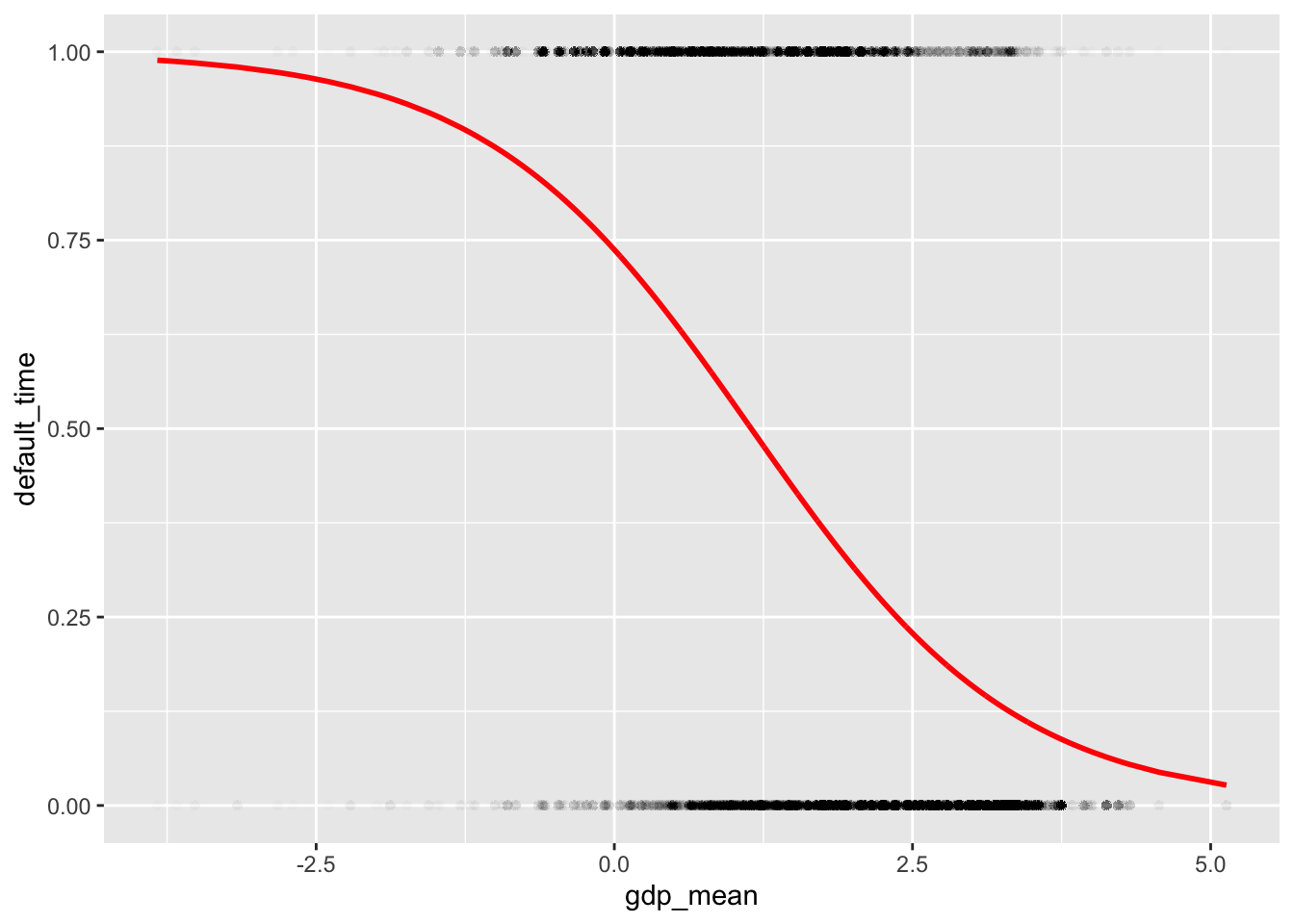
pattern: As gdp mean increases roughly from 3.75 to 5.0, the default rate shows a decrease pattern from 1 to 0. The dots are mainly gathered from 0 to 2.5 gdp mean for both default and pay-off.
Original House Price Index:
mor_mod1 <- glm(default_time ~ hpi_orig_time, data = mortgage_all, family = binomial)
(beta <- coef(mor_mod1))
## (Intercept) hpi_orig_time
## -5.41944535 0.02425822library(modelr)
(grid <- mortgage_all %>% data_grid(hpi_orig_time) %>%
add_predictions(mor_mod1, type = "response"))## # A tibble: 87 x 2
## hpi_orig_time pred
## <dbl> <dbl>
## 1 75.7 0.0270
## 2 75.7 0.0271
## 3 75.9 0.0272
## 4 76.4 0.0275
## 5 76.5 0.0275
## 6 76.5 0.0275
## 7 76.7 0.0277
## 8 76.9 0.0278
## 9 77.0 0.0279
## 10 77 0.0279
## # … with 77 more rowsggplot(mortgage_all, aes(hpi_orig_time)) + geom_point(aes(y = default_time),alpha = 0.005) +
geom_line(aes(y = pred), data = grid, color = "red", size = 1)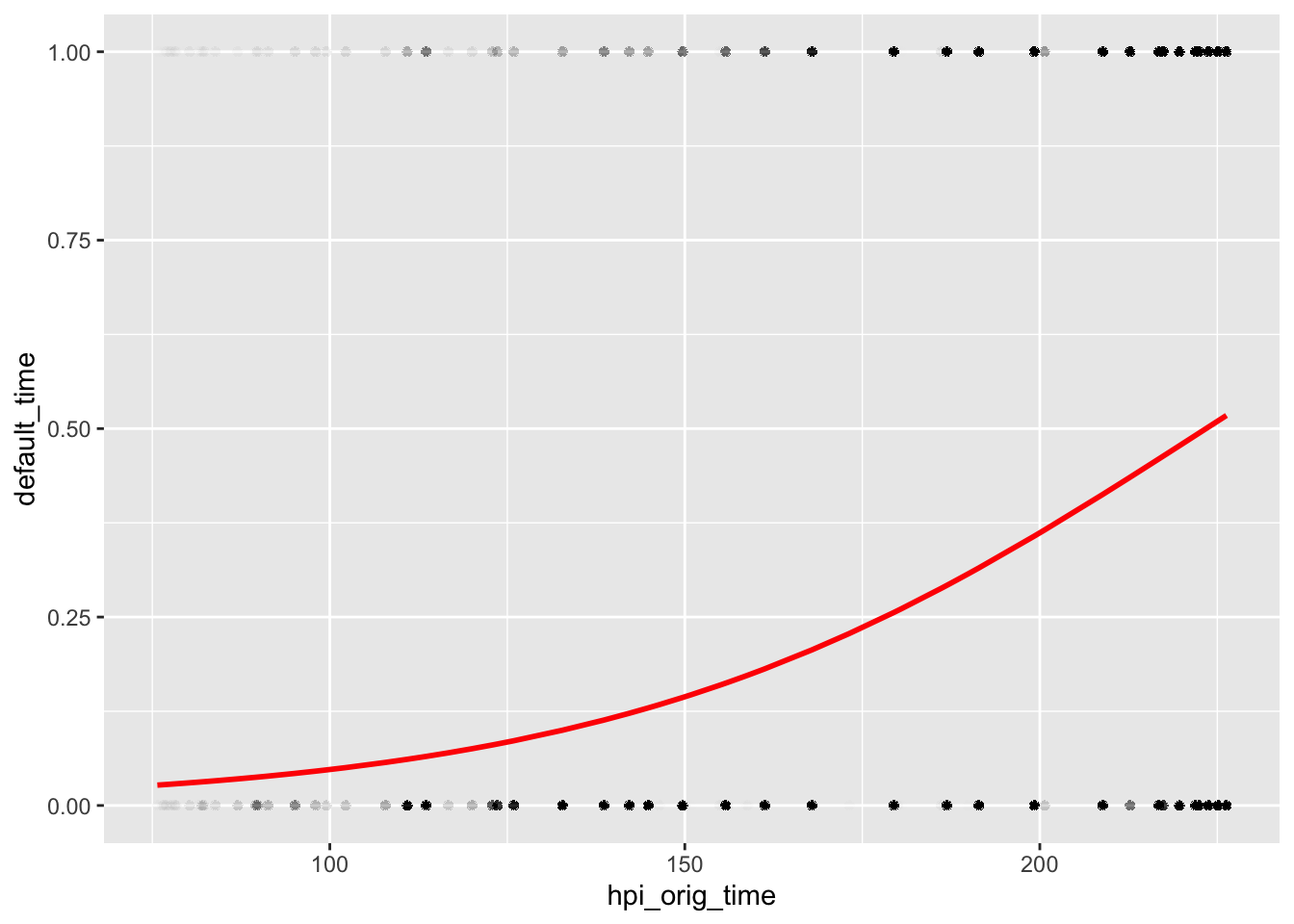
pattern: There is a weak correlation between the original house price index (base year = 100) and default rate. As the original house price index increases from 75 to 200, the default rate increases at the same time from 0 to 0.5.
For time varible, I will keep only origin time of the dataset:
mor_mod2 <- glm(default_time ~ orig_time, data = mortgage_all, family = binomial)
(beta <- coef(mor_mod2))
## (Intercept) orig_time
## -3.1697610 0.1243071library(modelr)
(grid <- mortgage_all %>% data_grid(orig_time) %>%
add_predictions(mor_mod2, type = "response"))## # A tibble: 88 x 2
## orig_time pred
## <dbl> <dbl>
## 1 -40 0.000291
## 2 -39 0.000329
## 3 -37 0.000422
## 4 -36 0.000478
## 5 -33 0.000694
## 6 -30 0.00101
## 7 -29 0.00114
## 8 -28 0.00129
## 9 -26 0.00166
## 10 -25 0.00187
## # … with 78 more rowsggplot(mortgage_all, aes(orig_time)) + geom_point(aes(y = default_time),alpha = 0.005) +
geom_line(aes(y = pred), data = grid, color = "red", size = 1)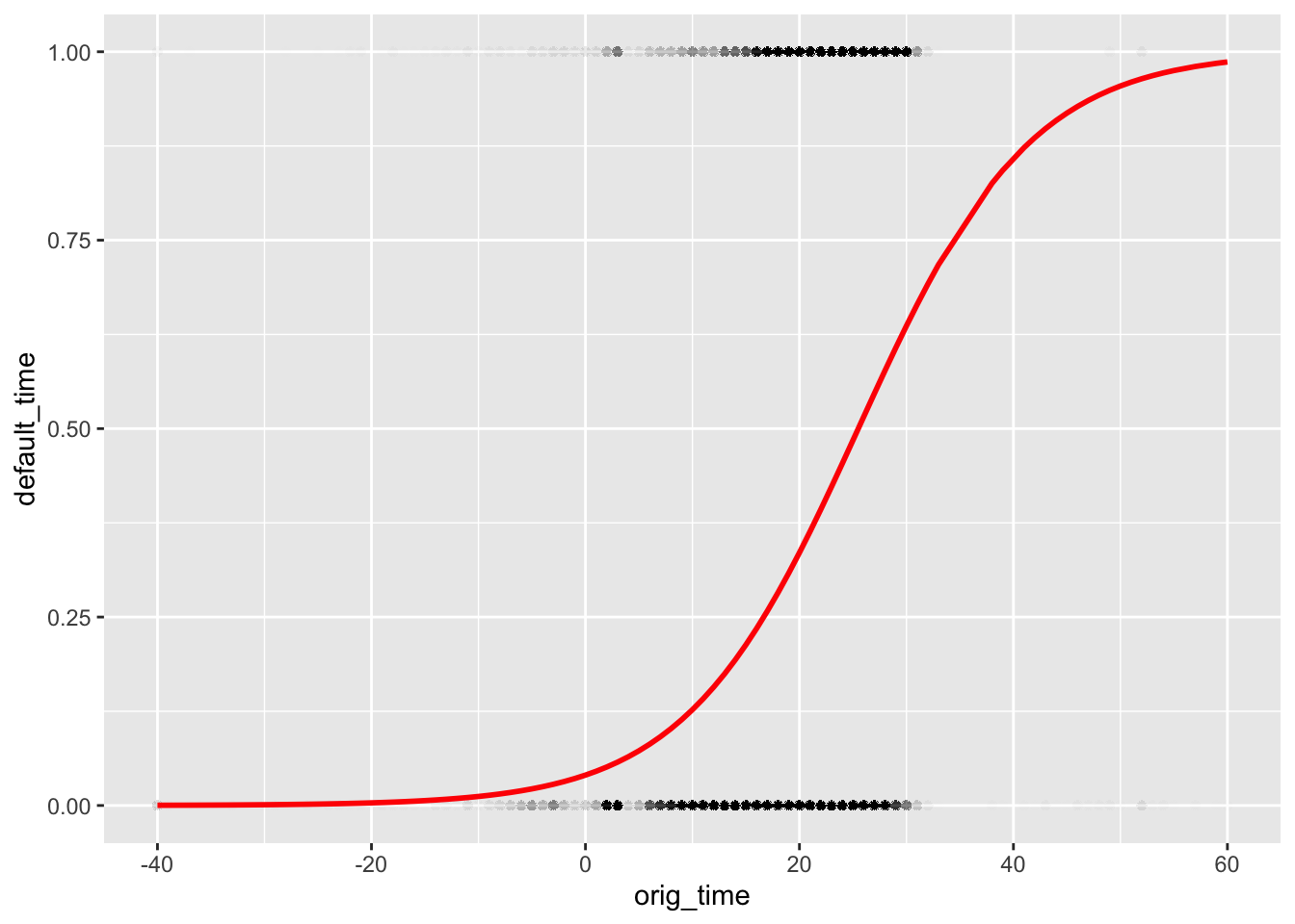
pattern: As we can see, the default rate tends to be 0 when time stamp for start of the mortgage from -40 to 0. The default rate increases dramatically from 0 to 40, and remains at 1 from 40 to 60.
First time Risk-free rate:
mor_mod4 <- glm(default_time ~ rate_time, data = mortgage_all, family = binomial)
(beta <- coef(mor_mod4))
## (Intercept) rate_time
## -4.2555650 0.8188854library(modelr)
(grid <- mortgage_all %>% data_grid(rate_time) %>%
add_predictions(mor_mod4, type = "response"))## # A tibble: 81 x 2
## rate_time pred
## <dbl> <dbl>
## 1 1.65 0.0519
## 2 1.67 0.0527
## 3 1.78 0.0574
## 4 1.87 0.0616
## 5 1.89 0.0625
## 6 1.92 0.0640
## 7 1.94 0.0650
## 8 2.17 0.0774
## 9 2.23 0.0810
## 10 2.52 0.100
## # … with 71 more rowsggplot(mortgage_all, aes(rate_time)) + geom_point(aes(y = default_time),alpha = 0.005) +
geom_line(aes(y = pred), data = grid, color = "red", size = 1)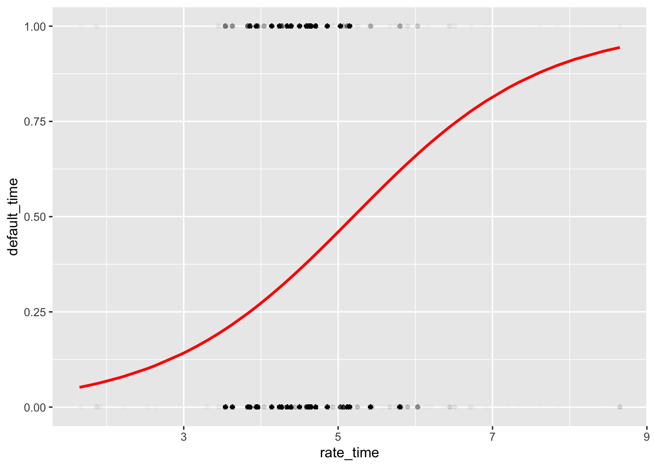
Pattern: There is a strong correlation between these two variables. As first time risk-free rate increases, the default rate increases dramatically from 0 to 1.
Unemployment Rate:
mor_mod5 <- glm(default_time ~ uer_mean, data = mortgage_all, family = binomial)
(beta <- coef(mor_mod5))
## (Intercept) uer_mean
## -2.5602844 0.3632487library(modelr)
(grid <- mortgage_all %>% data_grid(uer_mean) %>%
add_predictions(mor_mod5, type = "response"))## # A tibble: 1,113 x 2
## uer_mean pred
## <dbl> <dbl>
## 1 3.8 0.235
## 2 3.9 0.242
## 3 3.95 0.245
## 4 3.98 0.247
## 5 4 0.248
## 6 4.03 0.251
## 7 4.05 0.252
## 8 4.06 0.252
## 9 4.12 0.257
## 10 4.15 0.259
## # … with 1,103 more rowsggplot(mortgage_all, aes(uer_mean)) + geom_point(aes(y = default_time),alpha = 0.005) +
geom_line(aes(y = pred), data = grid, color = "red", size = 1)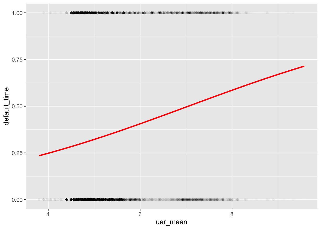
Pattern: There is a positive linear relationship between the average unemployment rate and default rate. As the average unemployment rate increases from roughly 4 to 10, the default rate increases from 0.25 to 0.75.
Mean Interest Rate:
mor_mod6 <- glm(default_time ~ interest_rate_mean, data = mortgage_all, family = binomial)
(beta <- coef(mor_mod6))
## (Intercept) interest_rate_mean
## -1.9736370 0.1906897library(modelr)
(grid <- mortgage_all %>% data_grid(interest_rate_mean) %>%
add_predictions(mor_mod6, type = "response"))## # A tibble: 7,527 x 2
## interest_rate_mean pred
## <dbl> <dbl>
## 1 1.12 0.147
## 2 1.72 0.162
## 3 1.75 0.162
## 4 1.99 0.169
## 5 1.99 0.169
## 6 2.00 0.169
## 7 2 0.169
## 8 2.00 0.169
## 9 2.01 0.169
## 10 2.02 0.170
## # … with 7,517 more rowsggplot(mortgage_all, aes(interest_rate_mean)) + geom_point(aes(y = default_time),alpha = 0.005) +
geom_line(aes(y = pred), data = grid, color = "red", size = 1)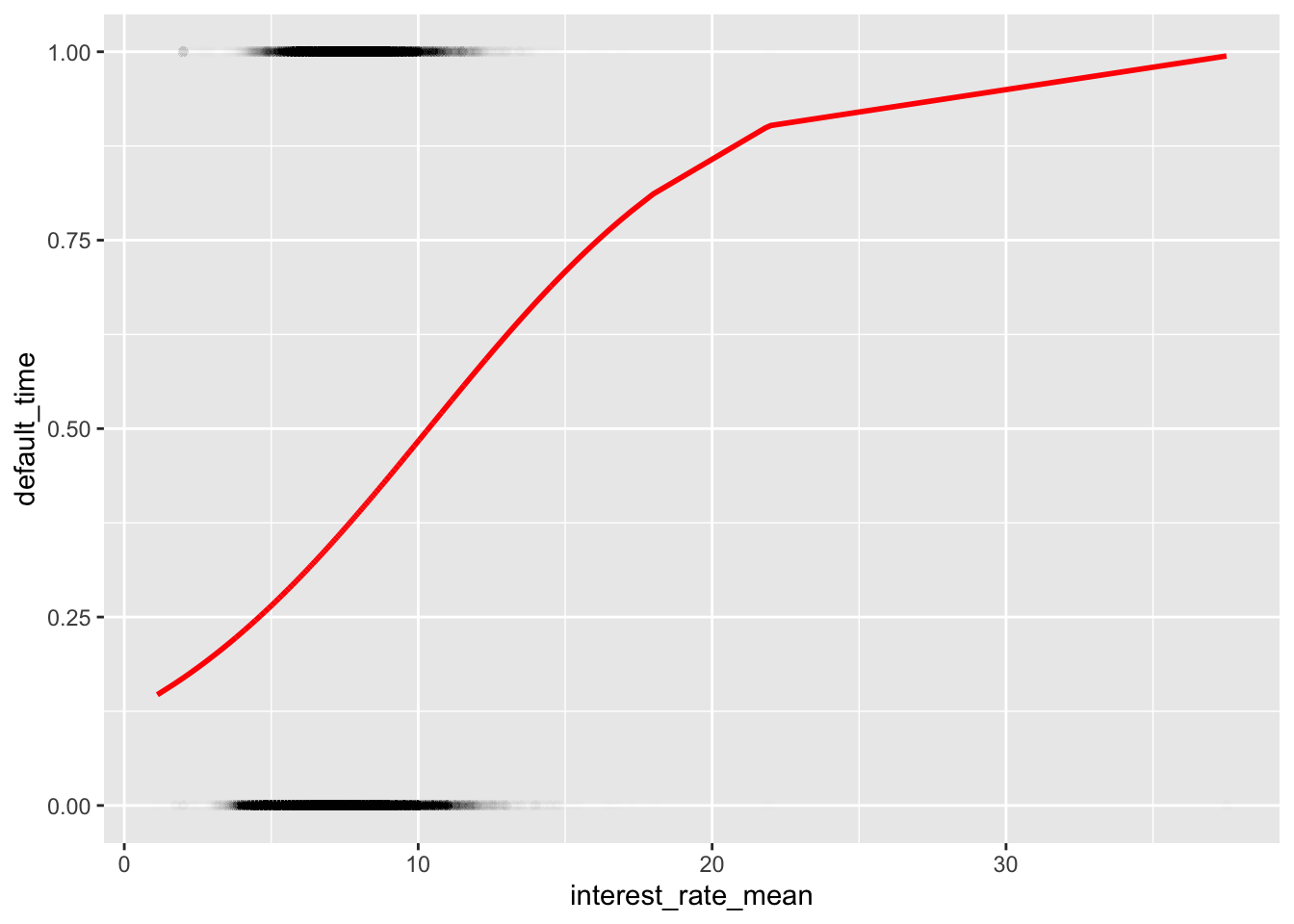
Pattern: The default rate increases dramatically as the average interest rate of all observation periods from roughly 2 to 20, and default rate tends to be flat from 20 to roughly 37.
Time to Maturity:
mor_mod7 <- glm(default_time ~ TTM, data = mortgage_all, family = binomial)
(beta <- coef(mor_mod7))
## (Intercept) TTM
## -3.22550171 0.02253902library(modelr)
(grid <- mortgage_all %>% data_grid(TTM) %>%
add_predictions(mor_mod7, type = "response"))## # A tibble: 146 x 2
## TTM pred
## <dbl> <dbl>
## 1 5 0.0426
## 2 9 0.0464
## 3 10 0.0474
## 4 11 0.0484
## 5 13 0.0506
## 6 14 0.0517
## 7 15 0.0528
## 8 16 0.0539
## 9 17 0.0551
## 10 18 0.0563
## # … with 136 more rowsggplot(mortgage_all, aes(TTM)) + geom_point(aes(y = default_time),alpha = 0.005) +
geom_line(aes(y = pred), data = grid, color = "red", size = 1)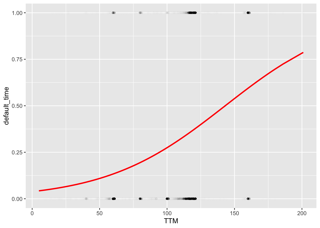
Pattern: There is a positive non-linear relationship between scheduled time to maturity and default rate. The slope increases slowly at the beginning, and start to increase relative deeply at roughly 100.
FICO score(credit score):
mor_mod8 <- glm(default_time ~ FICO_orig_time, data = mortgage_all, family = binomial)
(beta <- coef(mor_mod8))
## (Intercept) FICO_orig_time
## 1.497799187 -0.003128735library(modelr)
(grid <- mortgage_all %>% data_grid(FICO_orig_time) %>%
add_predictions(mor_mod8, type = "response"))## # A tibble: 389 x 2
## FICO_orig_time pred
## <dbl> <dbl>
## 1 400 0.561
## 2 406 0.557
## 3 413 0.551
## 4 420 0.546
## 5 428 0.540
## 6 429 0.539
## 7 433 0.536
## 8 439 0.531
## 9 441 0.529
## 10 442 0.529
## # … with 379 more rowsggplot(mortgage_all, aes(FICO_orig_time)) + geom_point(aes(y = default_time),alpha = 0.005) +
geom_line(aes(y = pred), data = grid, color = "red", size = 1)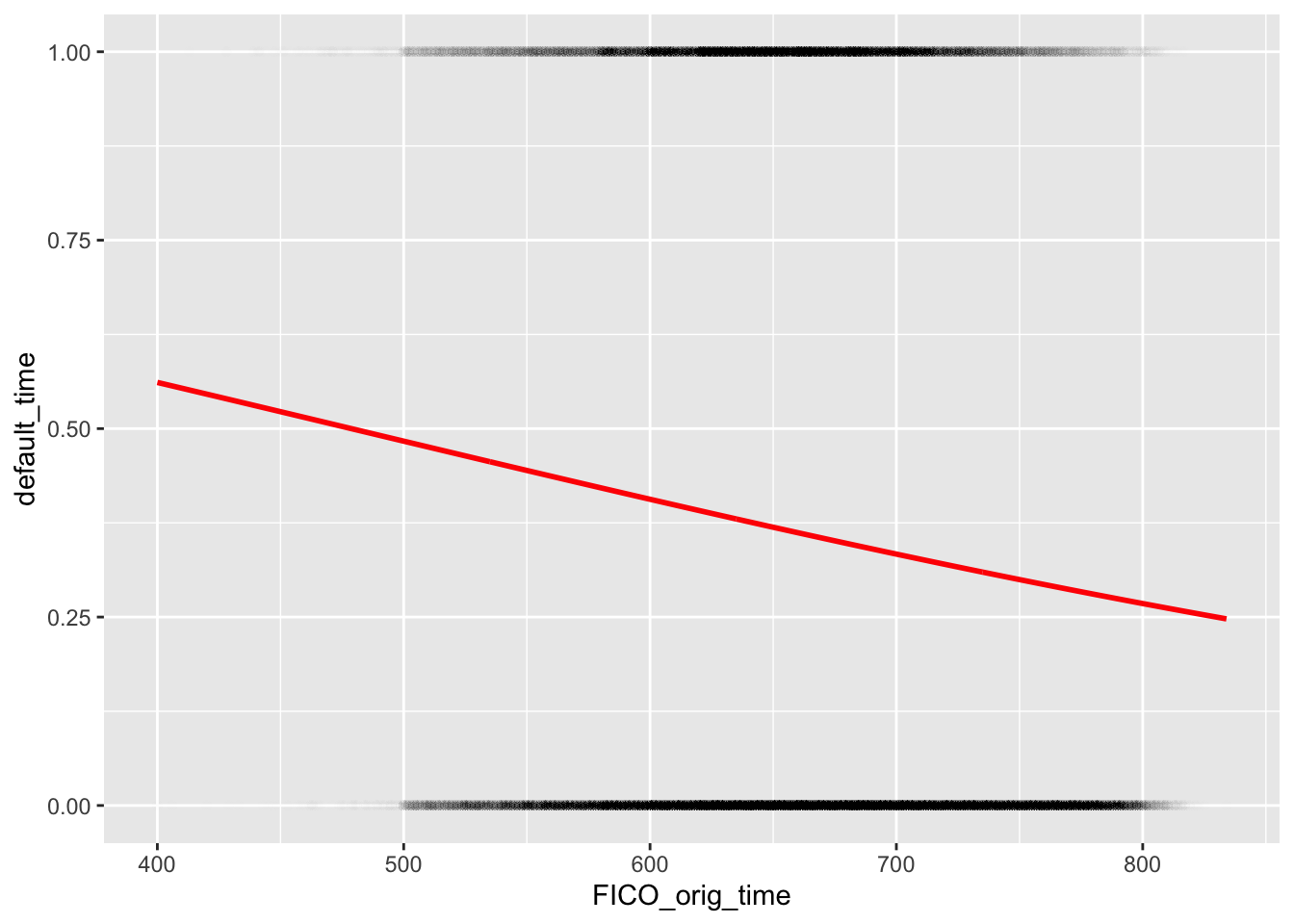
pattern: The correlation between default rate and FICO score(credit score) at origination time is negative and weak, which indicates a small correlation between these two variables.
Loan to Value ratio:
mor_mod9 <- glm(default_time ~ LTV_orig_time, data = mortgage_all, family = binomial)
(beta <- coef(mor_mod9))
## (Intercept) LTV_orig_time
## -2.09611716 0.01917789library(modelr)
(grid <- mortgage_all %>% data_grid(LTV_orig_time) %>%
add_predictions(mor_mod9, type = "response"))## # A tibble: 538 x 2
## LTV_orig_time pred
## <dbl> <dbl>
## 1 50.1 0.243
## 2 50.2 0.244
## 3 50.3 0.244
## 4 50.4 0.244
## 5 50.5 0.245
## 6 50.6 0.245
## 7 50.7 0.245
## 8 50.8 0.246
## 9 50.9 0.246
## 10 51 0.246
## # … with 528 more rowsggplot(mortgage_all, aes(LTV_orig_time)) + geom_point(aes(y = default_time),alpha = 0.005) +
geom_line(aes(y = pred), data = grid, color = "red", size = 1)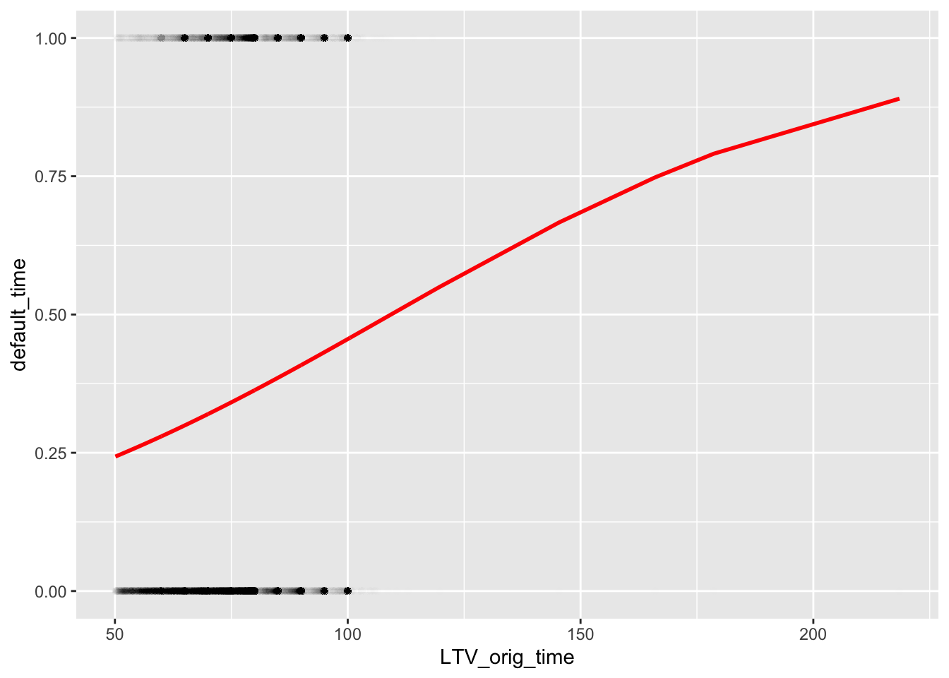
Pattern: The correlation here looks pretty steady, except a little twit around LTV_orig_time = 175. This indicates an overall stable positive linear correlation between default time and loan-to-value ratio.
age of a mortgage:
mor_mod10 <- glm(default_time ~ age, data = mortgage_all, family = binomial)
(beta <- coef(mor_mod10))
## (Intercept) age
## -0.49817484 -0.01776127library(modelr)
(grid <- mortgage_all %>% data_grid(age) %>%
add_predictions(mor_mod10, type = "response"))## # A tibble: 66 x 2
## age pred
## <dbl> <dbl>
## 1 0 0.378
## 2 1 0.374
## 3 2 0.370
## 4 3 0.366
## 5 4 0.361
## 6 5 0.357
## 7 6 0.353
## 8 7 0.349
## 9 8 0.345
## 10 9 0.341
## # … with 56 more rowsggplot(mortgage_all, aes(age)) + geom_point(aes(y = default_time),alpha = 0.005) +
geom_line(aes(y = pred), data = grid, color = "red", size = 1)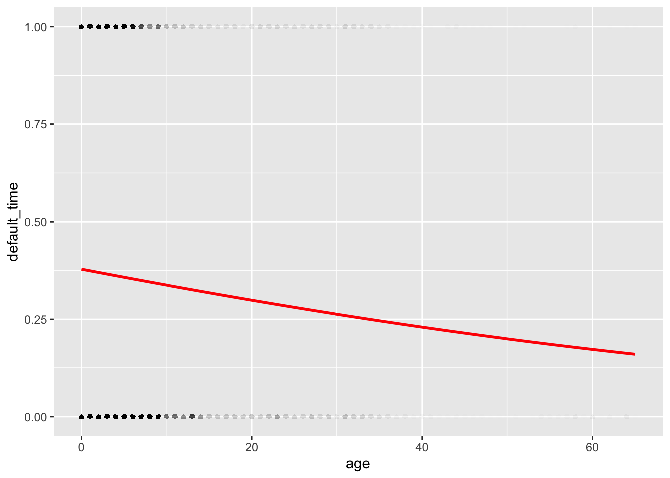
pattern: The correlation here looks negatively linear but not strong, since the correlation line is relatively flat, which indicates a small tangent and small correlation between these two variables.
Investor Type:
ggplot(data=mortgage_all, mapping=aes(x= investor_orig_time,y=REtype_SF_orig_time))+
  geom_bar(stat="identity")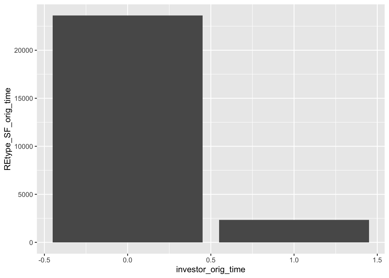
Pattern:
Value of the house:
mor_mod12 <- glm(default_time ~ balance_orig_time, data = mortgage_all, family = binomial)
(beta <- coef(mor_mod12))
## (Intercept) balance_orig_time
## -5.567810e-01 -1.075221e-08library(modelr)
(grid <- mortgage_all %>% data_grid(balance_orig_time) %>%
add_predictions(mor_mod12, type = "response"))## # A tibble: 9,409 x 2
## balance_orig_time pred
## <dbl> <dbl>
## 1 0 0.364
## 2 6246 0.364
## 3 9575 0.364
## 4 10000 0.364
## 5 10465. 0.364
## 6 11100 0.364
## 7 11400 0.364
## 8 11845. 0.364
## 9 12000 0.364
## 10 12008 0.364
## # … with 9,399 more rowsggplot(mortgage_all, aes(balance_orig_time)) + geom_point(aes(y = default_time),alpha = 0.005) +
geom_line(aes(y = pred), data = grid, color = "red", size = 1)
Pattern: There is almost no correlation between value of the house and default rate. The correlation line is totally flat, which means value of the house does not affect default time.
REtype_CO_orig_tim:condominium:
ggplot(data=mortgage_all, mapping=aes(x=default_time,y=REtype_CO_orig_time))+
  geom_bar(stat="identity")
Pattern: The ratio of pay-off to default in condominium is around 1:2, with pay-off approximately 1000 and default approximately 2000. This type of real estate has the largest difference in ratio between payoff and default.
REtype_PU_orig_time real estate type planned urban developments:
ggplot(data=mortgage_all, mapping=aes(x=default_time,y=REtype_PU_orig_time))+
  geom_bar(stat="identity")
Pattern: The ratio of pay-off to default in planned urban developments is around 3:5, with pay-off approximately 1800 and default approximately 3000.
REtype_SF_orig_time single family home:
ggplot(data=mortgage_all, mapping=aes(x=default_time,y=REtype_SF_orig_time))+
  geom_bar(stat="identity")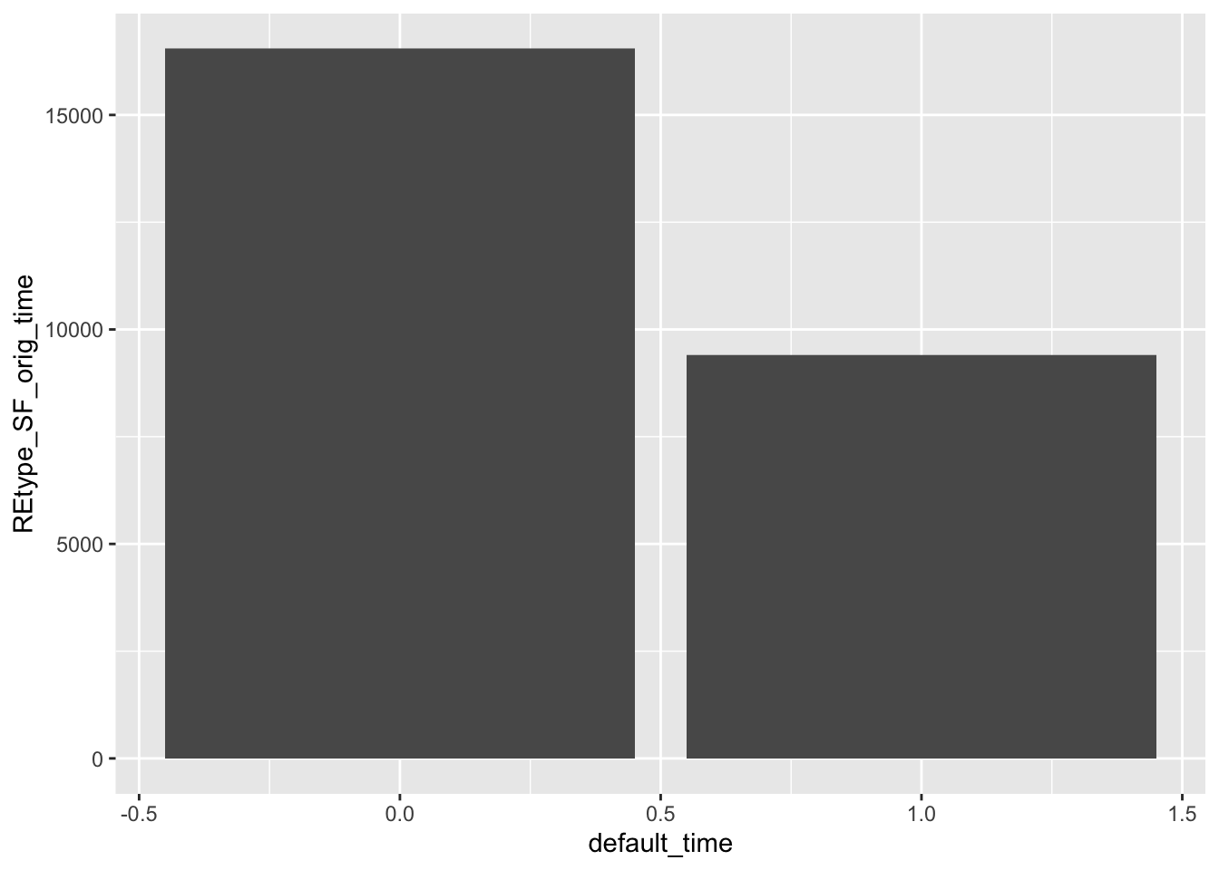
Pattern: The ratio of pay-off to default in single family home is around 19:33, with pay-off approximately 9500 and default approximately 16500. This type of real estate has the most counts. So, after ploting all these varible, we are now able to complete our full regression model:
library(modelr)
glm(default_time ~ age + first_time+REtype_CO_orig_time+REtype_PU_orig_time+REtype_SF_orig_time+
interest_rate_mean+gdp_mean+rate_time+hpi_orig_time+uer_mean+investor_orig_time+balance_orig_time+FICO_orig_time+LTV_orig_time+TTM- 1 , data = mortgage_all, family = binomial) %>% broom::tidy()
## # A tibble: 15 x 5
## term estimate std.error statistic p.value
## <chr> <dbl> <dbl> <dbl> <dbl>
## 1 age -1.91e-2 0.00502 -3.81 1.38e- 4
## 2 first_time 2.27e-2 0.00489 4.65 3.35e- 6
## 3 REtype_CO_orig_time -1.05e-2 0.0540 -0.194 8.46e- 1
## 4 REtype_PU_orig_time 7.95e-2 0.0446 1.78 7.48e- 2
## 5 REtype_SF_orig_time -8.40e-2 0.0315 -2.67 7.62e- 3
## 6 interest_rate_mean 7.94e-2 0.00858 9.25 2.29e- 20
## 7 gdp_mean -9.64e-1 0.0145 -66.3 0
## 8 rate_time 8.65e-2 0.0287 3.01 2.62e- 3
## 9 hpi_orig_time 5.48e-3 0.000974 5.62 1.89e- 8
## 10 uer_mean -1.44e-1 0.0128 -11.2 3.14e- 29
## 11 investor_orig_time 4.06e-1 0.0391 10.4 3.20e- 25
## 12 balance_orig_time -5.74e-9 0.0000000641 -0.0895 9.29e- 1
## 13 FICO_orig_time -6.32e-3 0.000185 -34.2 2.96e-256
## 14 LTV_orig_time 2.34e-2 0.00130 18.1 3.16e- 73
## 15 TTM 1.39e-2 0.000991 14.0 1.22e- 44As we can see from the chart, condominium or not, planned urban developments or not, the value of the house, is not statistically significant. Therefore, we will kick them out od our model.
library(modelr)
glm(default_time ~ age + first_time+REtype_SF_orig_time+interest_rate_mean+gdp_mean+rate_time+hpi_orig_time+uer_mean+investor_orig_time+FICO_orig_time+LTV_orig_time+TTM- 1 , data = mortgage_all, family = binomial) %>% broom::tidy()
## # A tibble: 12 x 5
## term estimate std.error statistic p.value
## <chr> <dbl> <dbl> <dbl> <dbl>
## 1 age -0.0192 0.00500 -3.85 1.18e- 4
## 2 first_time 0.0226 0.00486 4.65 3.27e- 6
## 3 REtype_SF_orig_time -0.107 0.0249 -4.29 1.82e- 5
## 4 interest_rate_mean 0.0786 0.00846 9.29 1.58e- 20
## 5 gdp_mean -0.964 0.0145 -66.3 0
## 6 rate_time 0.0880 0.0287 3.07 2.13e- 3
## 7 hpi_orig_time 0.00549 0.000973 5.64 1.68e- 8
## 8 uer_mean -0.144 0.0128 -11.2 3.52e- 29
## 9 investor_orig_time 0.401 0.0383 10.5 1.34e- 25
## 10 FICO_orig_time -0.00631 0.000179 -35.3 7.50e-273
## 11 LTV_orig_time 0.0235 0.00128 18.4 1.39e- 75
## 12 TTM 0.0140 0.000987 14.1 2.31e- 45Generally speaking, GDP growth, uemployment rate,and the mean interest rate is still the outside dominant factor that may influence one’s default rate. In addition to that, investor house or not, loan to house value ratio, time to maturity are also the inside factor that determines one’s default rate.Therefore, whether one will default or not in a mortgage is strongly related to both the economy of the country and the types of specific mortgage.