Mortgage Market analysis in the US
This dataset is from http://www.deepcreditrisk.com/data--code-private.html
Description:
The data set is in panel form and reports origination and performance observations for 50000 residential U.S. mortgage borrowers over 60 peiords. The periods have been deidentified. As in the real world, loans may originate before the start of the observation period. The loan observations may thus be censored as the loans mature or borrowers refinance. The data set is a randomized selection of mortgage-loan-level data collected from the portfolios underlying U.S. residential mortgage-backed securities (RMBS) securitization portfolios. Such randomization gives us a fair representation of US mortgage market development. We would like to combine the dataset with other market indicator to further measure the probability of default for personal investors.
Key variables include:
library(tidyverse)## ── Attaching packages ─────────────────────────────────────── tidyverse 1.3.1 ──## ✓ ggplot2 3.3.5 ✓ purrr 0.3.4
## ✓ tibble 3.1.2 ✓ dplyr 1.0.7
## ✓ tidyr 1.1.4 ✓ stringr 1.4.0
## ✓ readr 2.0.1 ✓ forcats 0.5.1## ── Conflicts ────────────────────────────────────────── tidyverse_conflicts() ──
## x dplyr::filter() masks stats::filter()
## x dplyr::lag() masks stats::lag()str<-'id: borrower id
time: time stamp of observation
orig_time: time stamp for origination
first_time: time stamp for first observation
mat_time: time stamp for maturity
res_time: time stamp for resolution
balance_time: outstanding balance at observation time
LTV_time: loan to value ratio at observation time, in %
interest_rate_time: interest rate at observation time, in %
rate_time: risk-free rate
hpi_time: house price index at observation time, base year=100
gdp_time: GDP growth at observation time, in %
uer_time: unemployment rate at observation time, in %
REtype_CO_orig_time: real estate type condominium: 1, otherwise: 0
REtype_PU_orig_time: real estate type planned urban developments: 1, otherwise: 0
REtype_SF_orig_time: single family home: 1, otherwise: 0
investor_orig_time: investor borrower: 1, otherwise: 0
balance_orig_time: outstanding balance at origination time
FICO_orig_time: FICO score at origination time, in %
LTV_orig_time: loan to value ratio at origination time, in %
Interest_Rate_orig_time: interest rate at origination time, in %
state_orig_time: US state in which the property is located
hpi_orig_time: house price index at observation time, base year=100
default_time: default observation at observation time
payoff_time: payoff observation at observation time
status_time: default (1), payoff (2) and non-default/non-payoff (0) observation at observation time
lgd_time: LGD assuming no discounting of cash flows
recovery_res: sum of all cash flows received during resolution period'
lista<-str_split(str, "\n")
keydataname<-data.frame(lista)
colnames(keydataname)<-'dataname'
keydataname<-keydataname %>% separate(dataname,into=c('Column Name','Description'),sep=':')## Warning: Expected 2 pieces. Additional pieces discarded in 4 rows [14, 15, 16,
## 17].print(as.tibble(keydataname), n = 28)## Warning: `as.tibble()` was deprecated in tibble 2.0.0.
## Please use `as_tibble()` instead.
## The signature and semantics have changed, see `?as_tibble`.## # A tibble: 28 x 2
## `Column Name` Description
## <chr> <chr>
## 1 id " borrower id"
## 2 time " time stamp of observation"
## 3 orig_time " time stamp for origination"
## 4 first_time " time stamp for first observation"
## 5 mat_time " time stamp for maturity"
## 6 res_time " time stamp for resolution"
## 7 balance_time " outstanding balance at observation time"
## 8 LTV_time " loan to value ratio at observation time, in %"
## 9 interest_rate_time " interest rate at observation time, in %"
## 10 rate_time " risk-free rate"
## 11 hpi_time " house price index at observation time, base year=100"
## 12 gdp_time " GDP growth at observation time, in %"
## 13 uer_time " unemployment rate at observation time, in %"
## 14 REtype_CO_orig_time " real estate type condominium"
## 15 REtype_PU_orig_time " real estate type planned urban developments"
## 16 REtype_SF_orig_time " single family home"
## 17 investor_orig_time " investor borrower"
## 18 balance_orig_time " outstanding balance at origination time"
## 19 FICO_orig_time " FICO score at origination time, in %"
## 20 LTV_orig_time " loan to value ratio at origination time, in %"
## 21 Interest_Rate_orig_… " interest rate at origination time, in %"
## 22 state_orig_time " US state in which the property is located"
## 23 hpi_orig_time " house price index at observation time, base year=100"
## 24 default_time " default observation at observation time"
## 25 payoff_time " payoff observation at observation time"
## 26 status_time " default (1), payoff (2) and non-default/non-payoff (0…
## 27 lgd_time " LGD assuming no discounting of cash flows"
## 28 recovery_res " sum of all cash flows received during resolution peri…The blog posts together should address the following topics.
Data Loading and Cleaning
library(tidyverse)
mortgage <-read_csv("dcr_full.csv", col_types=cols(
  id = col_double(),
  time = col_double(),
  orig_time = col_double(),
  first_time = col_double(),
  mat_time = col_double(),
  res_time = col_double(),
  balance_time = col_double(),
  LTV_time = col_double(),
  interest_rate_time = col_double(),
  rate_time = col_double(),
  hpi_time = col_double(),
  gdp_time = col_double(),
  uer_time = col_double(),
  REtype_CO_orig_time = col_double(),
  iREtype_PU_orig_time = col_double(),
  REtype_SF_orig_time = col_double(),
  investor_orig_time = col_double(),
  balance_orig_time = col_double(),
  FICO_orig_time = col_double(),
  LTV_orig_time = col_double(),
  Interest_Rate_orig_time = col_double(),
  state_orig_time = col_character(),
  hpi_orig_time = col_double(),
  default_time = col_double(),
  payoff_time = col_double(),
  status_time = col_character()
  ))
## Warning: The following named parsers don't match the column names:
## iREtype_PU_orig_timemortgage## # A tibble: 622,489 x 28
## id time orig_time first_time mat_time res_time balance_time LTV_time
## <dbl> <dbl> <dbl> <dbl> <dbl> <dbl> <dbl> <dbl>
## 1 1 25 -7 25 113 NA 41303. 24.5
## 2 1 26 -7 25 113 NA 41062. 24.5
## 3 1 27 -7 25 113 NA 40804. 24.6
## 4 1 28 -7 25 113 NA 40484. 24.7
## 5 1 29 -7 25 113 NA 40367. 24.9
## 6 1 30 -7 25 113 NA 40128. 25.3
## 7 1 31 -7 25 113 NA 39719. 26.6
## 8 1 32 -7 25 113 NA 35877. 25.9
## 9 1 33 -7 25 113 NA 34410. 25.6
## 10 1 34 -7 25 113 NA 33590. 26.0
## # … with 622,479 more rows, and 20 more variables: interest_rate_time <dbl>,
## # rate_time <dbl>, hpi_time <dbl>, gdp_time <dbl>, uer_time <dbl>,
## # REtype_CO_orig_time <dbl>, REtype_PU_orig_time <dbl>,
## # REtype_SF_orig_time <dbl>, investor_orig_time <dbl>,
## # balance_orig_time <dbl>, FICO_orig_time <dbl>, LTV_orig_time <dbl>,
## # Interest_Rate_orig_time <dbl>, state_orig_time <chr>, hpi_orig_time <dbl>,
## # default_time <dbl>, payoff_time <dbl>, status_time <chr>, lgd_time <dbl>,
## # recovery_res <dbl>problems()If you are working with a large data set, you might decide to start with a subset of the data. How did you choose this?
I use a random number generator because I do not want my subset to be biased and stratified.
Discuss any initial steps you are taking to load and clean the data.
Our Idea is to make a logistics regression to see any variable strongly influence people’s choice between payoff and default, so the first step for us to clean the data is to only select those who already reach the deadline (eliminate those have not reached the maturity) while 2 represents payoff, 1 represents default, what we do is to select only the status_time = 1 or 2
(mortgage <- mortgage %>% filter(status_time > 0))## # A tibble: 41,747 x 28
## id time orig_time first_time mat_time res_time balance_time LTV_time
## <dbl> <dbl> <dbl> <dbl> <dbl> <dbl> <dbl> <dbl>
## 1 1 48 -7 25 113 50 29087. 26.7
## 2 2 26 18 25 138 NA 105655. 65.5
## 3 3 29 -6 25 114 NA 44379. 31.5
## 4 5 27 18 25 138 NA 52101. 66.3
## 5 6 56 19 25 139 60 190474. 75.8
## 6 7 26 18 25 138 NA 107916. 77.9
## 7 8 25 18 25 138 NA 152393. 58.8
## 8 9 37 18 25 138 NA 130140. 99.1
## 9 10 29 18 25 139 34 88046. 67.3
## 10 11 27 18 25 138 NA 154664. 78.8
## # … with 41,737 more rows, and 20 more variables: interest_rate_time <dbl>,
## # rate_time <dbl>, hpi_time <dbl>, gdp_time <dbl>, uer_time <dbl>,
## # REtype_CO_orig_time <dbl>, REtype_PU_orig_time <dbl>,
## # REtype_SF_orig_time <dbl>, investor_orig_time <dbl>,
## # balance_orig_time <dbl>, FICO_orig_time <dbl>, LTV_orig_time <dbl>,
## # Interest_Rate_orig_time <dbl>, state_orig_time <chr>, hpi_orig_time <dbl>,
## # default_time <dbl>, payoff_time <dbl>, status_time <chr>, lgd_time <dbl>,
## # recovery_res <dbl>(mortgage %>% ggplot(aes(x = balance_time)) + geom_histogram())## `stat_bin()` using `bins = 30`. Pick better value with `binwidth`.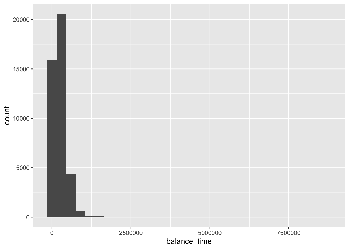
sqrt_result <- sqrt(var(mortgage$balance_time))
mean_result <-mean(mortgage$balance_time)
(threshold <- mean_result + 2 * sqrt_result)
## [1] 653053.3(mortgage <- mortgage %>% filter(balance_time < 422225.7))## # A tibble: 35,612 x 28
## id time orig_time first_time mat_time res_time balance_time LTV_time
## <dbl> <dbl> <dbl> <dbl> <dbl> <dbl> <dbl> <dbl>
## 1 1 48 -7 25 113 50 29087. 26.7
## 2 2 26 18 25 138 NA 105655. 65.5
## 3 3 29 -6 25 114 NA 44379. 31.5
## 4 5 27 18 25 138 NA 52101. 66.3
## 5 6 56 19 25 139 60 190474. 75.8
## 6 7 26 18 25 138 NA 107916. 77.9
## 7 8 25 18 25 138 NA 152393. 58.8
## 8 9 37 18 25 138 NA 130140. 99.1
## 9 10 29 18 25 139 34 88046. 67.3
## 10 11 27 18 25 138 NA 154664. 78.8
## # … with 35,602 more rows, and 20 more variables: interest_rate_time <dbl>,
## # rate_time <dbl>, hpi_time <dbl>, gdp_time <dbl>, uer_time <dbl>,
## # REtype_CO_orig_time <dbl>, REtype_PU_orig_time <dbl>,
## # REtype_SF_orig_time <dbl>, investor_orig_time <dbl>,
## # balance_orig_time <dbl>, FICO_orig_time <dbl>, LTV_orig_time <dbl>,
## # Interest_Rate_orig_time <dbl>, state_orig_time <chr>, hpi_orig_time <dbl>,
## # default_time <dbl>, payoff_time <dbl>, status_time <chr>, lgd_time <dbl>,
## # recovery_res <dbl>mortgage %>% ggplot(aes(x = balance_time)) + geom_histogram()## `stat_bin()` using `bins = 30`. Pick better value with `binwidth`.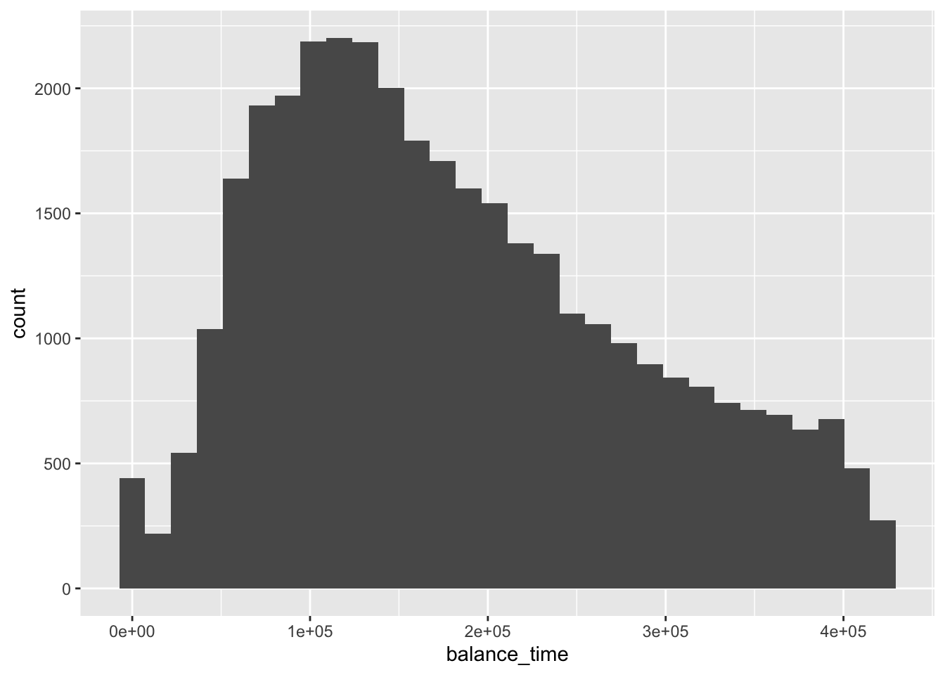
mortgage %>% ggplot(aes(x = status_time, y = balance_time)) + geom_boxplot()
mortgage %>% ggplot(aes(x = status_time, y = LTV_time)) + geom_boxplot()## Warning: Removed 12 rows containing non-finite values (stat_boxplot).
mortgage %>% ggplot(aes(x = status_time, y = interest_rate_time)) + geom_boxplot()
mortgage %>% ggplot(aes(x = status_time, y = Interest_Rate_orig_time)) + geom_boxplot()
mortgage %>% ggplot(aes(x = status_time, y = gdp_time)) + geom_boxplot()
mortgage %>% ggplot(aes(x = status_time, y = uer_time)) + geom_boxplot()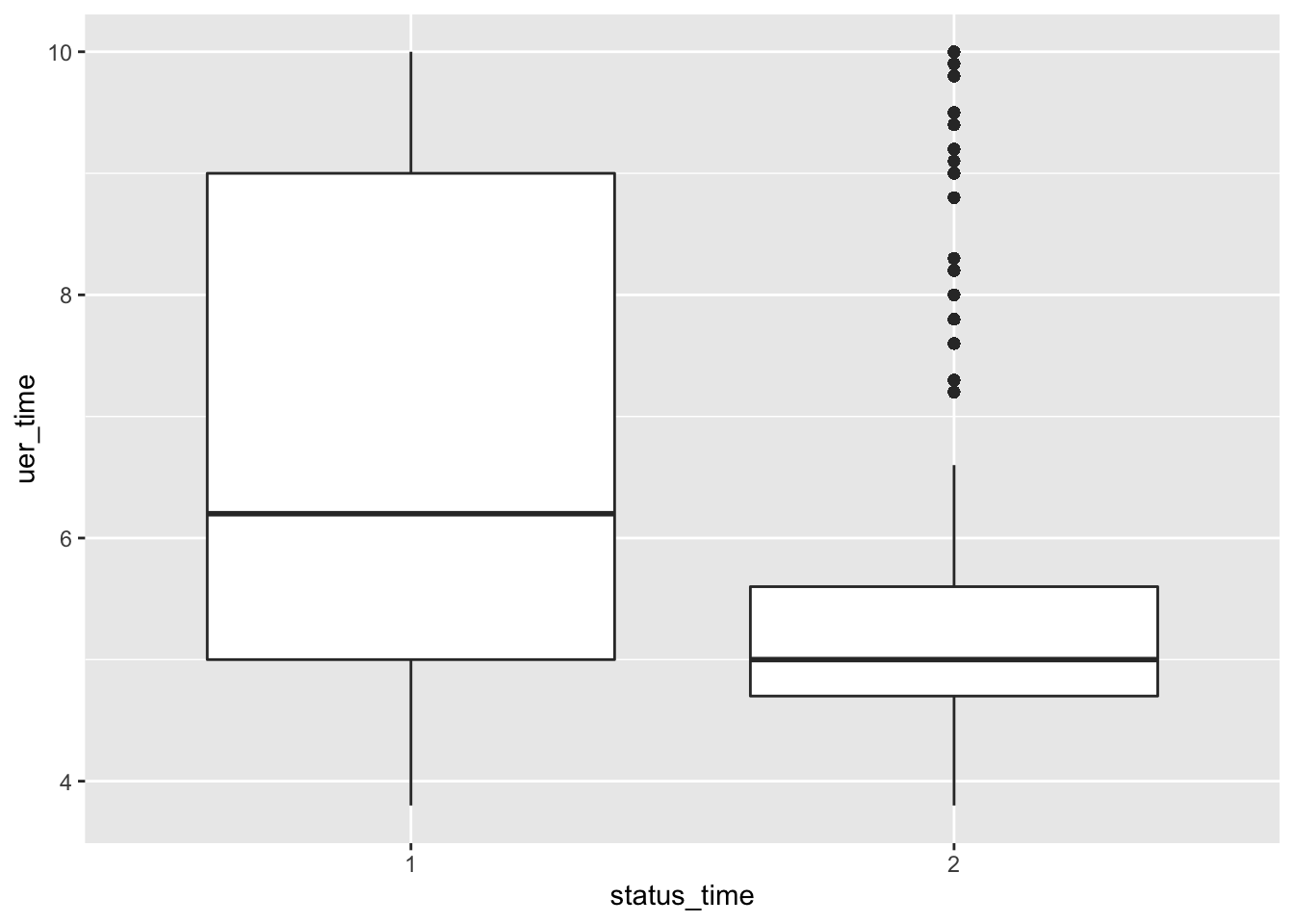 # If you are working with a large data set, you might decide to start with a subset of the data. How did you choose this?
mortgage %>% mutate(count = n())%>% mutate(random = runif(count,1.0,10000.0)) %>% filter(random < 1000)## # A tibble: 3,542 x 30
## id time orig_time first_time mat_time res_time balance_time LTV_time
## <dbl> <dbl> <dbl> <dbl> <dbl> <dbl> <dbl> <dbl>
## 1 2 26 18 25 138 NA 105655. 65.5
## 2 9 37 18 25 138 NA 130140. 99.1
## 3 19 28 19 25 139 30 187753. 68.2
## 4 21 28 18 25 139 NA 197993. 67.9
## 5 29 33 18 25 139 38 177668. 80.0
## 6 32 25 19 25 139 NA 238082. 67.1
## 7 34 26 19 25 139 NA 257601. 67.4
## 8 62 36 25 33 140 NA 68553. 133.
## 9 68 38 25 33 141 NA 82984. 113.
## 10 73 41 25 33 140 NA 93837. 109.
## # … with 3,532 more rows, and 22 more variables: interest_rate_time <dbl>,
## # rate_time <dbl>, hpi_time <dbl>, gdp_time <dbl>, uer_time <dbl>,
## # REtype_CO_orig_time <dbl>, REtype_PU_orig_time <dbl>,
## # REtype_SF_orig_time <dbl>, investor_orig_time <dbl>,
## # balance_orig_time <dbl>, FICO_orig_time <dbl>, LTV_orig_time <dbl>,
## # Interest_Rate_orig_time <dbl>, state_orig_time <chr>, hpi_orig_time <dbl>,
## # default_time <dbl>, payoff_time <dbl>, status_time <chr>, lgd_time <dbl>,
## # recovery_res <dbl>, count <int>, random <dbl>mortgage %>% ggplot(aes(id)) + geom_freqpoly()## `stat_bin()` using `bins = 30`. Pick better value with `binwidth`.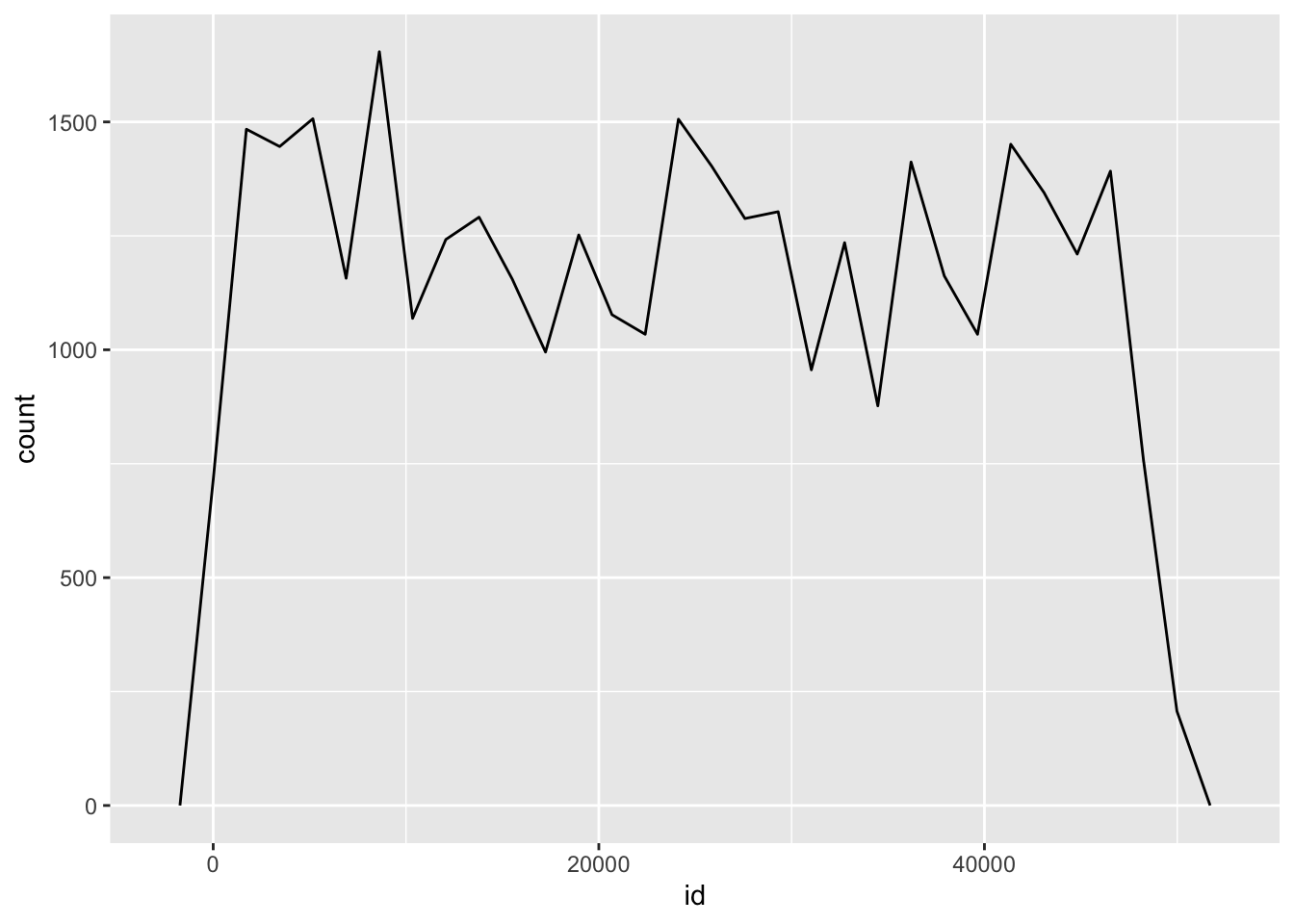
mortgage %>% count(time)## # A tibble: 60 x 2
## time n
## <dbl> <int>
## 1 1 22
## 2 2 37
## 3 3 57
## 4 4 56
## 5 5 65
## 6 6 95
## 7 7 80
## 8 8 72
## 9 9 97
## 10 10 74
## # … with 50 more rowsmortgage %>% count(orig_time)## # A tibble: 72 x 2
## orig_time n
## <dbl> <int>
## 1 -40 43
## 2 -39 3
## 3 -37 2
## 4 -36 1
## 5 -33 2
## 6 -30 3
## 7 -29 3
## 8 -28 2
## 9 -26 3
## 10 -25 2
## # … with 62 more rowsmortgage %>% count(first_time)## # A tibble: 41 x 2
## first_time n
## <dbl> <int>
## 1 1 276
## 2 2 267
## 3 3 387
## 4 4 16
## 5 5 24
## 6 6 102
## 7 9 135
## 8 10 71
## 9 11 175
## 10 12 313
## # … with 31 more rowsmortgage %>% count(mat_time)## # A tibble: 175 x 2
## mat_time n
## <dbl> <int>
## 1 23 1
## 2 26 1
## 3 27 1
## 4 28 1
## 5 29 4
## 6 30 1
## 7 31 3
## 8 32 4
## 9 33 2
## 10 34 3
## # … with 165 more rowsmortgage %>% count(res_time)## # A tibble: 58 x 2
## res_time n
## <dbl> <int>
## 1 4 3
## 2 5 2
## 3 6 5
## 4 7 7
## 5 8 4
## 6 9 11
## 7 10 9
## 8 11 11
## 9 12 16
## 10 13 14
## # … with 48 more rowsmortgage %>% ggplot(aes(balance_time)) + geom_histogram()## `stat_bin()` using `bins = 30`. Pick better value with `binwidth`.
mortgage %>% filter(balance_time < 0)## # A tibble: 0 x 28
## # … with 28 variables: id <dbl>, time <dbl>, orig_time <dbl>, first_time <dbl>,
## # mat_time <dbl>, res_time <dbl>, balance_time <dbl>, LTV_time <dbl>,
## # interest_rate_time <dbl>, rate_time <dbl>, hpi_time <dbl>, gdp_time <dbl>,
## # uer_time <dbl>, REtype_CO_orig_time <dbl>, REtype_PU_orig_time <dbl>,
## # REtype_SF_orig_time <dbl>, investor_orig_time <dbl>,
## # balance_orig_time <dbl>, FICO_orig_time <dbl>, LTV_orig_time <dbl>,
## # Interest_Rate_orig_time <dbl>, state_orig_time <chr>, hpi_orig_time <dbl>,
## # default_time <dbl>, payoff_time <dbl>, status_time <chr>, lgd_time <dbl>,
## # recovery_res <dbl>mortgage %>% count(LTV_time)## # A tibble: 32,926 x 2
## LTV_time n
## <dbl> <int>
## 1 0 285
## 2 0.0430 1
## 3 0.0462 1
## 4 0.0554 1
## 5 0.0939 1
## 6 0.112 1
## 7 0.133 1
## 8 0.143 1
## 9 0.148 1
## 10 0.169 1
## # … with 32,916 more rowsmortgage %>% ggplot(aes(LTV_time)) + geom_histogram()## `stat_bin()` using `bins = 30`. Pick better value with `binwidth`.## Warning: Removed 12 rows containing non-finite values (stat_bin).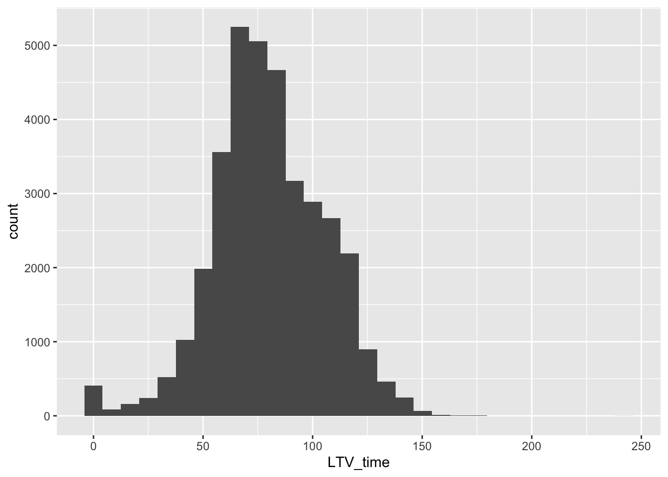
mortgage %>% count(LTV_time, balance_time)## # A tibble: 35,263 x 3
## LTV_time balance_time n
## <dbl> <dbl> <int>
## 1 0 0 285
## 2 0.0430 351. 1
## 3 0.0462 24.9 1
## 4 0.0554 455. 1
## 5 0.0939 262. 1
## 6 0.112 530. 1
## 7 0.133 1271. 1
## 8 0.143 673. 1
## 9 0.148 229 1
## 10 0.169 1508. 1
## # … with 35,253 more rowsmortgage %>% ggplot(aes(interest_rate_time)) + geom_histogram()## `stat_bin()` using `bins = 30`. Pick better value with `binwidth`.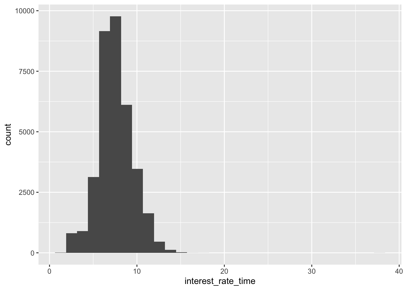
mortgage %>% ggplot(aes(rate_time)) + geom_histogram()## `stat_bin()` using `bins = 30`. Pick better value with `binwidth`.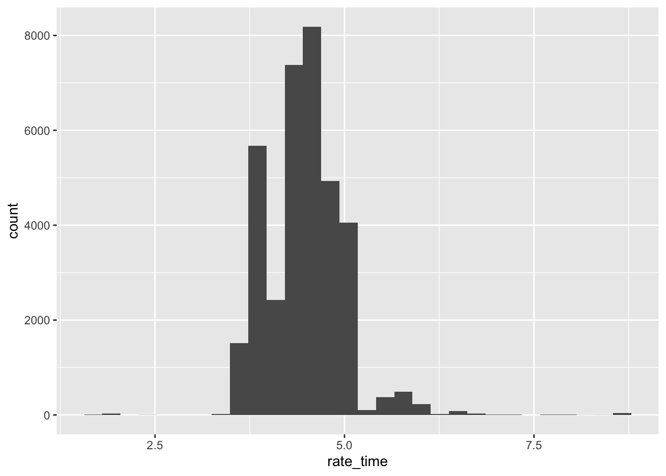
mortgage %>% ggplot(aes(hpi_time)) + geom_histogram()## `stat_bin()` using `bins = 30`. Pick better value with `binwidth`.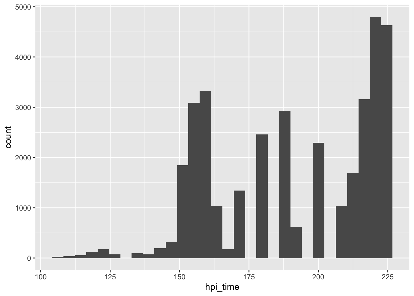
mortgage %>% ggplot(aes(hpi_orig_time)) + geom_histogram()## `stat_bin()` using `bins = 30`. Pick better value with `binwidth`.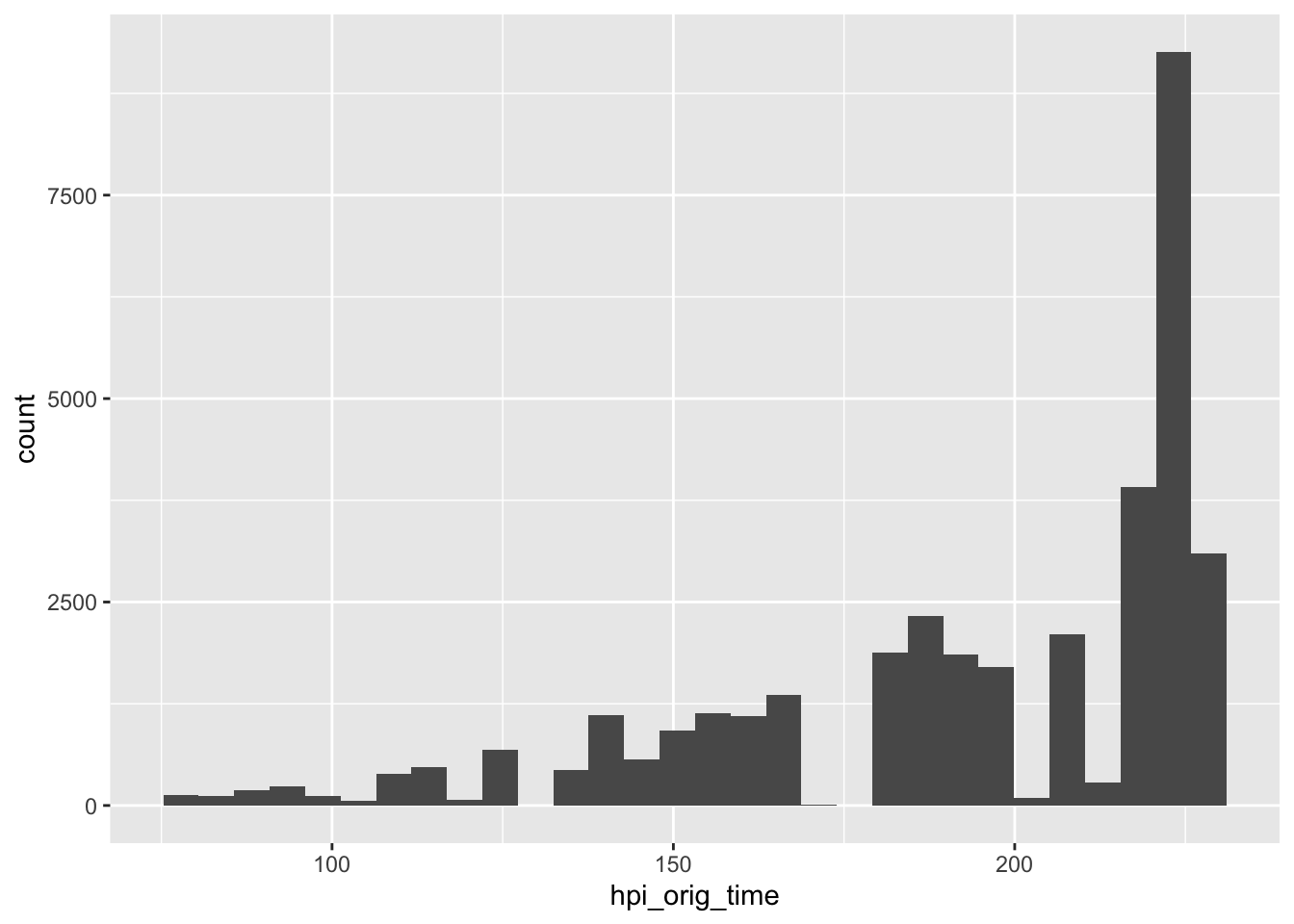
mortgage %>% ggplot(aes(gdp_time)) + geom_histogram()## `stat_bin()` using `bins = 30`. Pick better value with `binwidth`.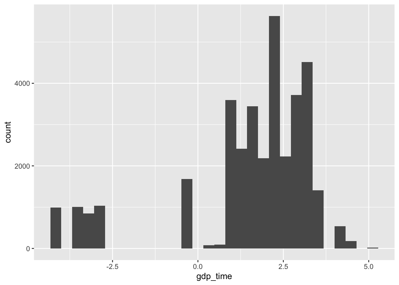
mortgage %>% ggplot(aes(uer_time)) + geom_histogram()## `stat_bin()` using `bins = 30`. Pick better value with `binwidth`.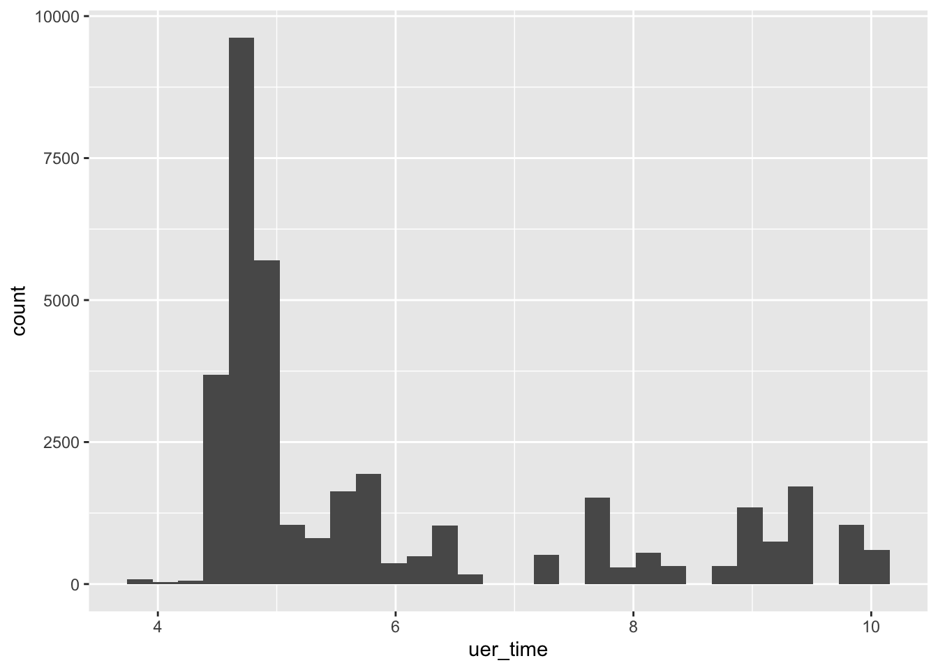
mortgage %>% count(REtype_CO_orig_time)## # A tibble: 2 x 2
## REtype_CO_orig_time n
## <dbl> <int>
## 1 0 33192
## 2 1 2420mortgage %>% count(REtype_PU_orig_time)## # A tibble: 2 x 2
## REtype_PU_orig_time n
## <dbl> <int>
## 1 0 31730
## 2 1 3882mortgage %>% count(REtype_SF_orig_time)## # A tibble: 2 x 2
## REtype_SF_orig_time n
## <dbl> <int>
## 1 0 13217
## 2 1 22395mortgage %>% count(investor_orig_time)## # A tibble: 2 x 2
## investor_orig_time n
## <dbl> <int>
## 1 0 31141
## 2 1 4471mortgage %>% ggplot(aes(balance_orig_time)) + geom_histogram()## `stat_bin()` using `bins = 30`. Pick better value with `binwidth`.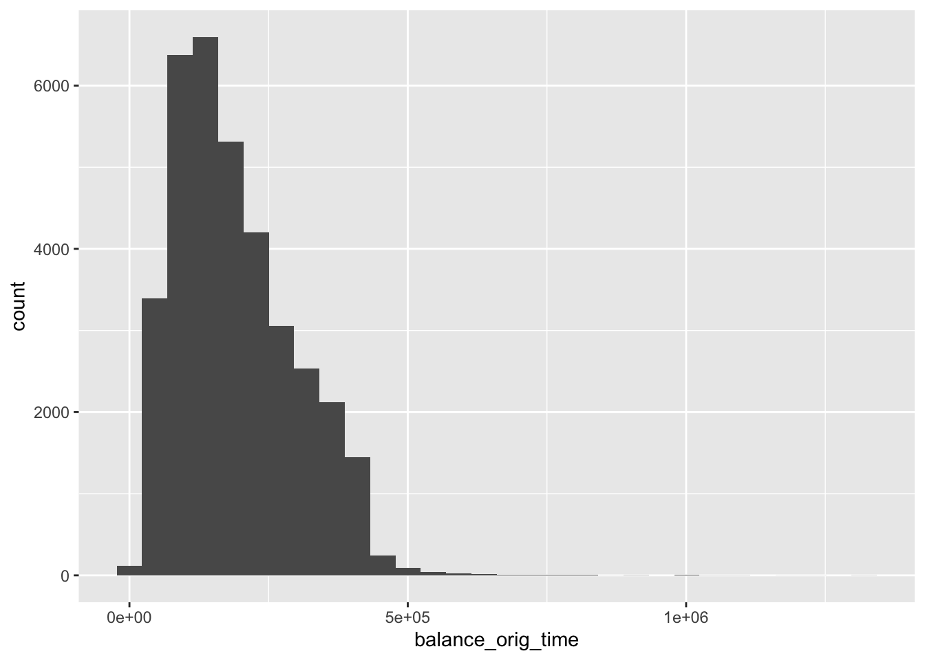
mortgage %>% filter(balance_time < 0)## # A tibble: 0 x 28
## # … with 28 variables: id <dbl>, time <dbl>, orig_time <dbl>, first_time <dbl>,
## # mat_time <dbl>, res_time <dbl>, balance_time <dbl>, LTV_time <dbl>,
## # interest_rate_time <dbl>, rate_time <dbl>, hpi_time <dbl>, gdp_time <dbl>,
## # uer_time <dbl>, REtype_CO_orig_time <dbl>, REtype_PU_orig_time <dbl>,
## # REtype_SF_orig_time <dbl>, investor_orig_time <dbl>,
## # balance_orig_time <dbl>, FICO_orig_time <dbl>, LTV_orig_time <dbl>,
## # Interest_Rate_orig_time <dbl>, state_orig_time <chr>, hpi_orig_time <dbl>,
## # default_time <dbl>, payoff_time <dbl>, status_time <chr>, lgd_time <dbl>,
## # recovery_res <dbl>mortgage %>% ggplot(aes(FICO_orig_time)) + geom_histogram()## `stat_bin()` using `bins = 30`. Pick better value with `binwidth`.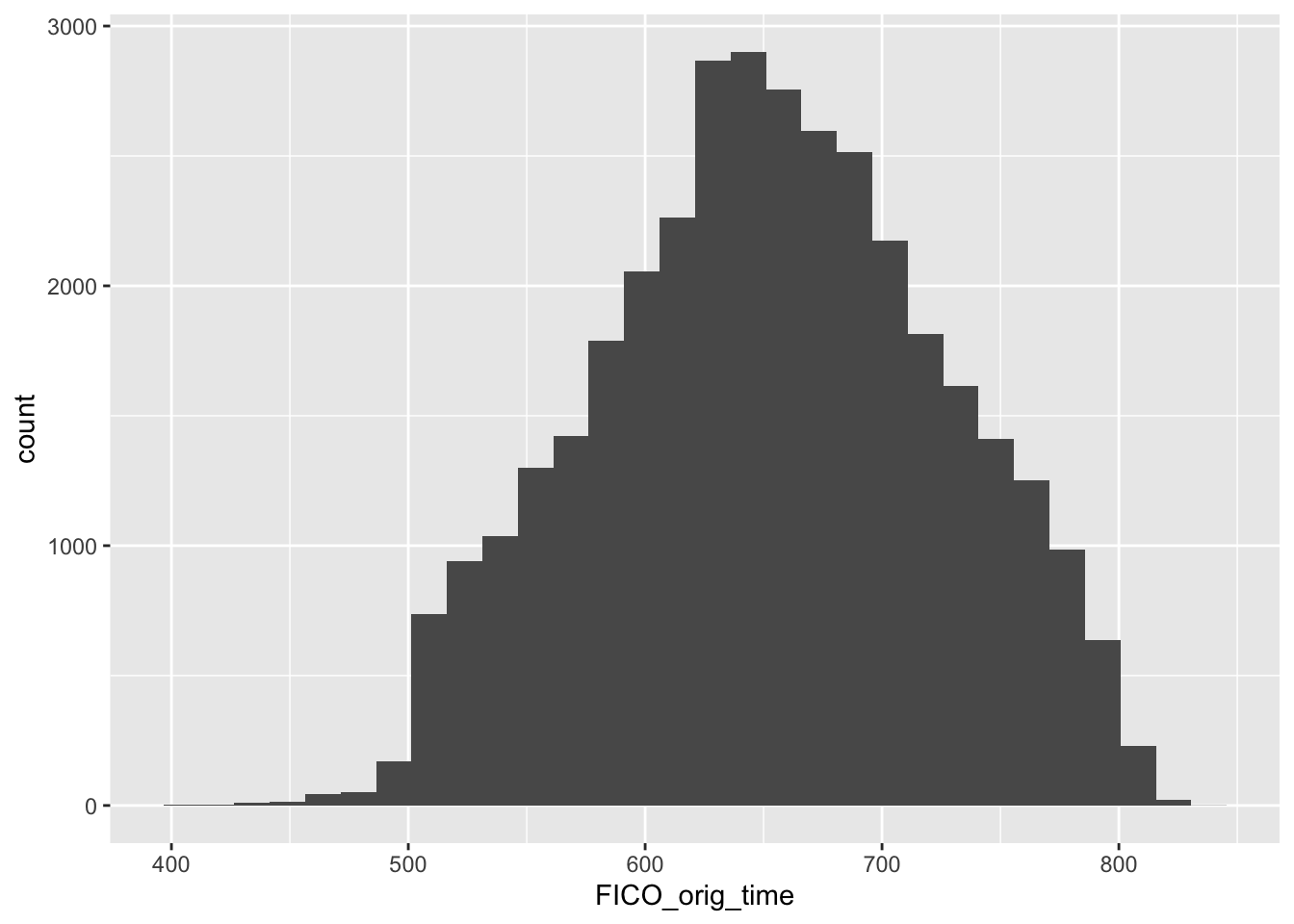
mortgage %>% ggplot(aes(LTV_orig_time)) + geom_histogram()## `stat_bin()` using `bins = 30`. Pick better value with `binwidth`.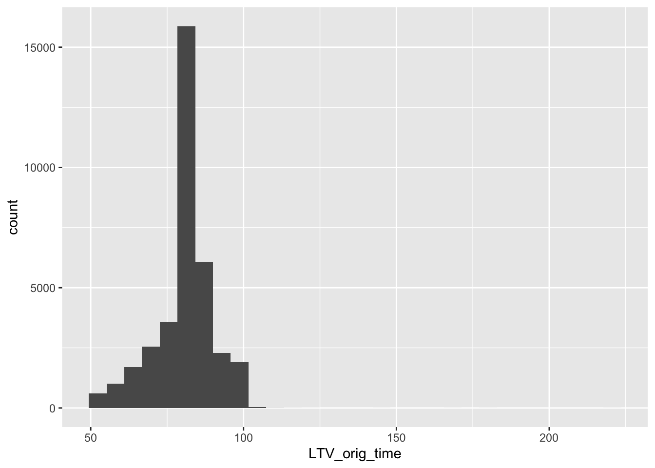
mortgage %>% ggplot(aes(Interest_Rate_orig_time)) + geom_histogram()## `stat_bin()` using `bins = 30`. Pick better value with `binwidth`.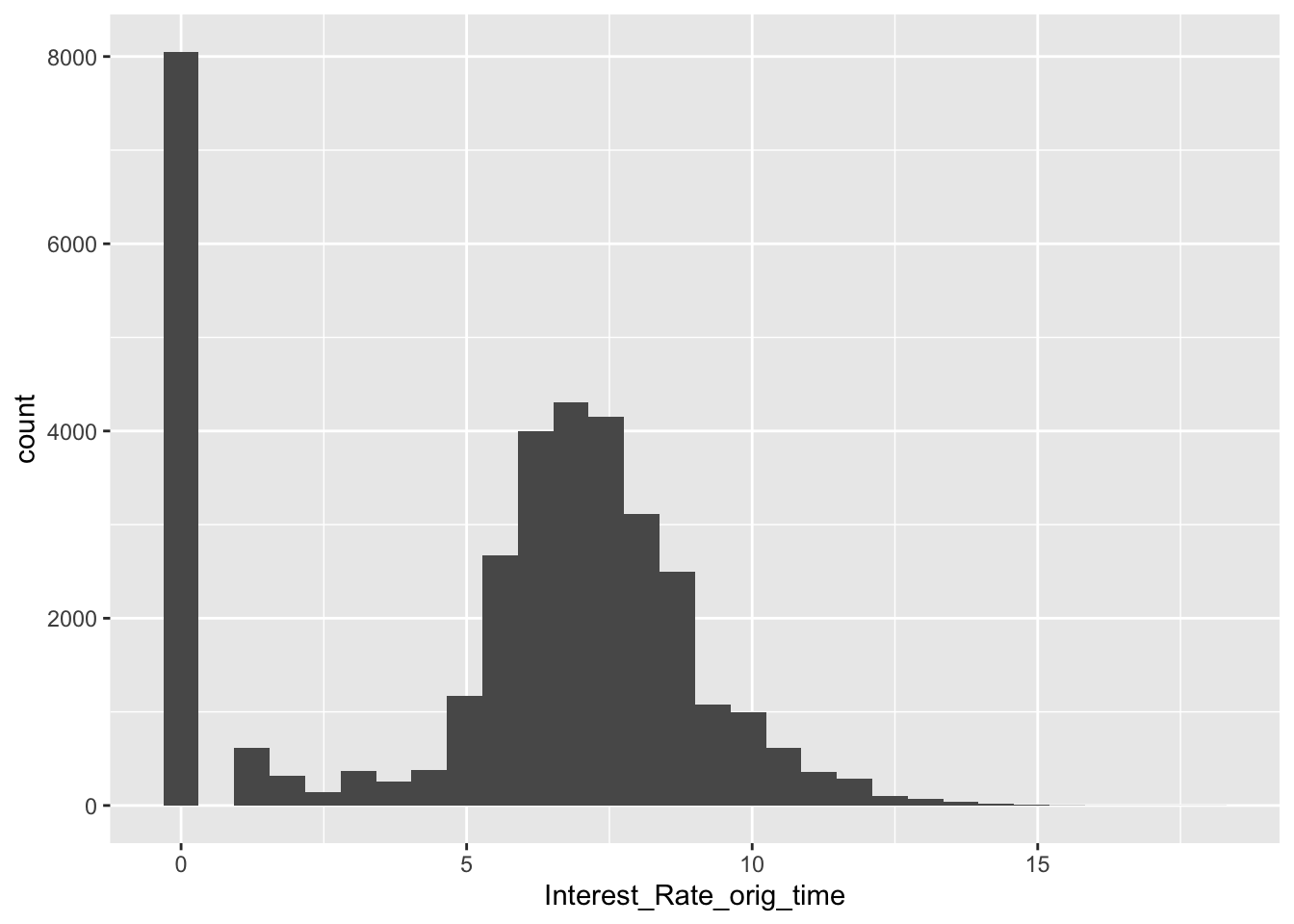
mortgage %>% filter(Interest_Rate_orig_time < 0)## # A tibble: 0 x 28
## # … with 28 variables: id <dbl>, time <dbl>, orig_time <dbl>, first_time <dbl>,
## # mat_time <dbl>, res_time <dbl>, balance_time <dbl>, LTV_time <dbl>,
## # interest_rate_time <dbl>, rate_time <dbl>, hpi_time <dbl>, gdp_time <dbl>,
## # uer_time <dbl>, REtype_CO_orig_time <dbl>, REtype_PU_orig_time <dbl>,
## # REtype_SF_orig_time <dbl>, investor_orig_time <dbl>,
## # balance_orig_time <dbl>, FICO_orig_time <dbl>, LTV_orig_time <dbl>,
## # Interest_Rate_orig_time <dbl>, state_orig_time <chr>, hpi_orig_time <dbl>,
## # default_time <dbl>, payoff_time <dbl>, status_time <chr>, lgd_time <dbl>,
## # recovery_res <dbl>mortgage %>% count(default_time)## # A tibble: 2 x 2
## default_time n
## <dbl> <int>
## 1 0 22825
## 2 1 12787mortgage %>% count(payoff_time)## # A tibble: 2 x 2
## payoff_time n
## <dbl> <int>
## 1 0 12787
## 2 1 22825mortgage %>% count(status_time)## # A tibble: 2 x 2
## status_time n
## <chr> <int>
## 1 1 12787
## 2 2 22825mortgage %>% count(state_orig_time)## # A tibble: 54 x 2
## state_orig_time n
## <chr> <int>
## 1 AK 23
## 2 AL 223
## 3 AR 110
## 4 AZ 1533
## 5 CA 6554
## 6 CO 828
## 7 CT 381
## 8 DC 87
## 9 DE 88
## 10 FL 3981
## # … with 44 more rowsmortage1 <- mortgage %>% filter(!is.na(state_orig_time))To clean the data, we use count function to check categorical value and geom_histogram to check numeral value. The Zero values in LTV and outstanding balance matches with each other(When the household pay off the debts). Since they are meaningful, we decide to leave them. Some of the variables like res_time has a lot of NA vlaues, but they are meaningful. We should keep them. However, there are 2829 NA values in state variable. Since they are meaningless, and the number is relatively small, we decided to filter them out.
One thing worths noticing is that the time of the dataset has been deidentified.It is difficult for us to combine ours with other datasets. Therefore, we decide to refill the exact time back. We do this by comparing the GDP growth data inside the dataset:
mortage1 %>% count(gdp_time,time) %>% ggplot(aes(time,gdp_time)) + geom_line()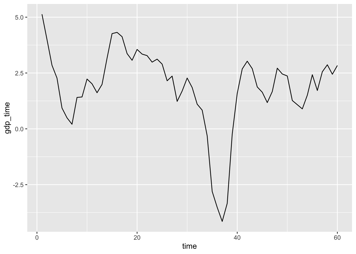
In US history, it is rare to see negative GDP growth. Therefore we check from the website and found out that the only peroid is US history with around -4.11% GDP growth, which is in the first quarter in 2009. After that, we compare other time and GDP growth, found out that the whole dataset is separated into 60 quaters from 2000 Q1 to 2014 Q4. Therefore, we can add the exact timeback to our dataset:
date_seq<-seq(as.Date("2000/03/31"), by = "quarter", length.out = 60)
date_dataframe<-data.frame(date_seq)
date_dataframe<- date_dataframe%>%separate(date_seq,into=c('year','month','day'),sep='-')
date_dataframe$quater=1
date_dataframe$quater[date_dataframe$month=='07']<-2
date_dataframe$quater[date_dataframe$month=='10']<-3
date_dataframe$quater[date_dataframe$month=='12']<-4
date_dataframe$time<-seq(1,60,1)
mortgage2 <- mortage1 %>% left_join(date_dataframe, by = "time")
mortgage2
## # A tibble: 35,449 x 32
## id time orig_time first_time mat_time res_time balance_time LTV_time
## <dbl> <dbl> <dbl> <dbl> <dbl> <dbl> <dbl> <dbl>
## 1 1 48 -7 25 113 50 29087. 26.7
## 2 2 26 18 25 138 NA 105655. 65.5
## 3 3 29 -6 25 114 NA 44379. 31.5
## 4 5 27 18 25 138 NA 52101. 66.3
## 5 6 56 19 25 139 60 190474. 75.8
## 6 7 26 18 25 138 NA 107916. 77.9
## 7 8 25 18 25 138 NA 152393. 58.8
## 8 9 37 18 25 138 NA 130140. 99.1
## 9 10 29 18 25 139 34 88046. 67.3
## 10 11 27 18 25 138 NA 154664. 78.8
## # … with 35,439 more rows, and 24 more variables: interest_rate_time <dbl>,
## # rate_time <dbl>, hpi_time <dbl>, gdp_time <dbl>, uer_time <dbl>,
## # REtype_CO_orig_time <dbl>, REtype_PU_orig_time <dbl>,
## # REtype_SF_orig_time <dbl>, investor_orig_time <dbl>,
## # balance_orig_time <dbl>, FICO_orig_time <dbl>, LTV_orig_time <dbl>,
## # Interest_Rate_orig_time <dbl>, state_orig_time <chr>, hpi_orig_time <dbl>,
## # default_time <dbl>, payoff_time <dbl>, status_time <chr>, lgd_time <dbl>,
## # recovery_res <dbl>, year <chr>, month <chr>, day <chr>, quater <dbl>After loading and cleaning, mortgage2 is the dataset we are working on.
(mortgage3 <- mortgage2 %>% filter(status_time > 0))## # A tibble: 35,449 x 32
## id time orig_time first_time mat_time res_time balance_time LTV_time
## <dbl> <dbl> <dbl> <dbl> <dbl> <dbl> <dbl> <dbl>
## 1 1 48 -7 25 113 50 29087. 26.7
## 2 2 26 18 25 138 NA 105655. 65.5
## 3 3 29 -6 25 114 NA 44379. 31.5
## 4 5 27 18 25 138 NA 52101. 66.3
## 5 6 56 19 25 139 60 190474. 75.8
## 6 7 26 18 25 138 NA 107916. 77.9
## 7 8 25 18 25 138 NA 152393. 58.8
## 8 9 37 18 25 138 NA 130140. 99.1
## 9 10 29 18 25 139 34 88046. 67.3
## 10 11 27 18 25 138 NA 154664. 78.8
## # … with 35,439 more rows, and 24 more variables: interest_rate_time <dbl>,
## # rate_time <dbl>, hpi_time <dbl>, gdp_time <dbl>, uer_time <dbl>,
## # REtype_CO_orig_time <dbl>, REtype_PU_orig_time <dbl>,
## # REtype_SF_orig_time <dbl>, investor_orig_time <dbl>,
## # balance_orig_time <dbl>, FICO_orig_time <dbl>, LTV_orig_time <dbl>,
## # Interest_Rate_orig_time <dbl>, state_orig_time <chr>, hpi_orig_time <dbl>,
## # default_time <dbl>, payoff_time <dbl>, status_time <chr>, lgd_time <dbl>,
## # recovery_res <dbl>, year <chr>, month <chr>, day <chr>, quater <dbl>mortgage2 %>% ggplot(aes(x = balance_time)) + geom_histogram(binwidth = 10000)
These are patterns we found:
sqrt_result <- sqrt(var(mortgage$balance_time))
mean_result <-mean(mortgage$balance_time)
(threshold <- mean_result + 2 * sqrt_result)
## [1] 387104.2(mortgage <- mortgage %>% filter(balance_time < 422225.7))## # A tibble: 35,612 x 28
## id time orig_time first_time mat_time res_time balance_time LTV_time
## <dbl> <dbl> <dbl> <dbl> <dbl> <dbl> <dbl> <dbl>
## 1 1 48 -7 25 113 50 29087. 26.7
## 2 2 26 18 25 138 NA 105655. 65.5
## 3 3 29 -6 25 114 NA 44379. 31.5
## 4 5 27 18 25 138 NA 52101. 66.3
## 5 6 56 19 25 139 60 190474. 75.8
## 6 7 26 18 25 138 NA 107916. 77.9
## 7 8 25 18 25 138 NA 152393. 58.8
## 8 9 37 18 25 138 NA 130140. 99.1
## 9 10 29 18 25 139 34 88046. 67.3
## 10 11 27 18 25 138 NA 154664. 78.8
## # … with 35,602 more rows, and 20 more variables: interest_rate_time <dbl>,
## # rate_time <dbl>, hpi_time <dbl>, gdp_time <dbl>, uer_time <dbl>,
## # REtype_CO_orig_time <dbl>, REtype_PU_orig_time <dbl>,
## # REtype_SF_orig_time <dbl>, investor_orig_time <dbl>,
## # balance_orig_time <dbl>, FICO_orig_time <dbl>, LTV_orig_time <dbl>,
## # Interest_Rate_orig_time <dbl>, state_orig_time <chr>, hpi_orig_time <dbl>,
## # default_time <dbl>, payoff_time <dbl>, status_time <chr>, lgd_time <dbl>,
## # recovery_res <dbl>mortgage %>% ggplot(aes(x = balance_time)) + geom_histogram()## `stat_bin()` using `bins = 30`. Pick better value with `binwidth`.
mortgage %>% ggplot(aes(x = status_time, y = balance_time)) + geom_boxplot()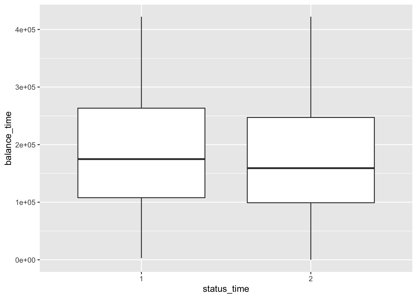
mortgage %>% ggplot(aes(x = status_time, y = LTV_time)) + geom_boxplot()## Warning: Removed 12 rows containing non-finite values (stat_boxplot).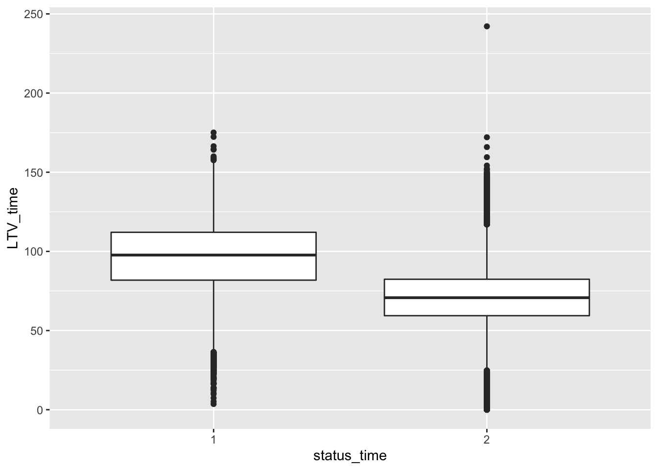
mortgage %>% ggplot(aes(x = status_time, y = interest_rate_time)) + geom_boxplot()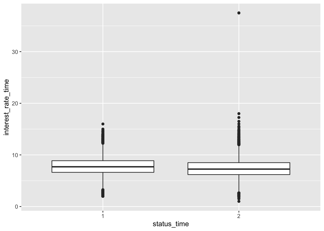
mortgage %>% ggplot(aes(x = status_time, y = Interest_Rate_orig_time)) + geom_boxplot()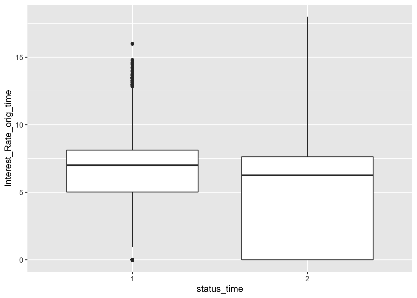
mortgage %>% ggplot(aes(x = status_time, y = gdp_time)) + geom_boxplot()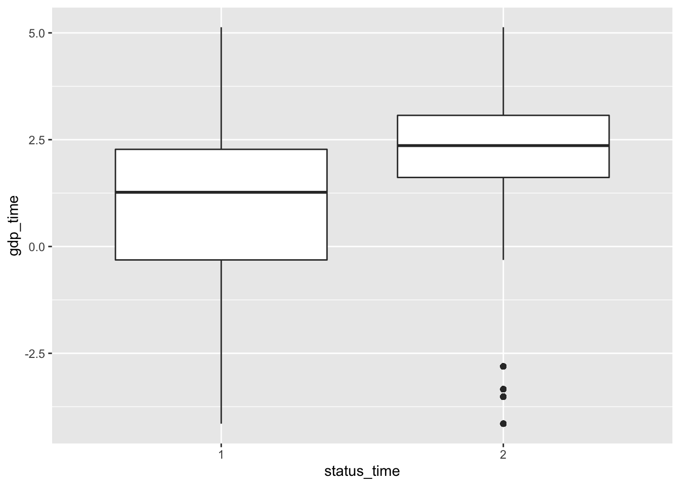
mortgage %>% ggplot(aes(x = status_time, y = uer_time)) + geom_boxplot()
Our Idea is to make a logistics regression to see any variable strongly influence people’s choice between payoff and default, so the first step for us to clean the data is to only select those who already reach the deadline (eliminate those have not reached the maturity) while 2 represents payoff, 1 represents default, what we do is to select only the status_time = 1 or 2
No big difference between payoff and default groups of status in outstanding balance, loan-to-value and interest rate at observation time. For interest rate at original time, the upper quartile and mean between payoff and default groups have no large difference, but the lower quartile of payoff group is apparently lower than the default group. The GDP at observation time for payoff group is apparently higher than default group. For the unemployment rate at observation time, both group have similar lower quartile, but default group has apparently higher mean and upper quartile than the payoff group.
Since this is a large dataset, we can start by a subset.We can use a random number generator because I do not want my subset to be biased and stratified.
mortgage %>% mutate(count = n())%>% mutate(random = runif(count,1.0,10000.0)) %>% filter(random < 1000)## # A tibble: 3,562 x 30
## id time orig_time first_time mat_time res_time balance_time LTV_time
## <dbl> <dbl> <dbl> <dbl> <dbl> <dbl> <dbl> <dbl>
## 1 23 25 18 25 139 NA 79980. 52.8
## 2 24 32 19 25 139 38 35166. 64.6
## 3 38 27 19 25 139 NA 218782. 67.7
## 4 50 27 19 25 139 NA 121370. 80.4
## 5 59 30 -15 25 105 NA 57423. 22.0
## 6 60 28 -13 25 107 NA 113538. 21.6
## 7 64 33 25 33 140 NA 0 0
## 8 81 26 21 25 141 NA 234598. 73.8
## 9 95 31 22 25 142 43 141288. 84.8
## 10 98 37 25 33 141 41 119337. 117.
## # … with 3,552 more rows, and 22 more variables: interest_rate_time <dbl>,
## # rate_time <dbl>, hpi_time <dbl>, gdp_time <dbl>, uer_time <dbl>,
## # REtype_CO_orig_time <dbl>, REtype_PU_orig_time <dbl>,
## # REtype_SF_orig_time <dbl>, investor_orig_time <dbl>,
## # balance_orig_time <dbl>, FICO_orig_time <dbl>, LTV_orig_time <dbl>,
## # Interest_Rate_orig_time <dbl>, state_orig_time <chr>, hpi_orig_time <dbl>,
## # default_time <dbl>, payoff_time <dbl>, status_time <chr>, lgd_time <dbl>,
## # recovery_res <dbl>, count <int>, random <dbl>