The blog posts together should address the following topics. Data Loading and Cleaning Discuss any initial steps you are taking to load and clean the data.
library(tidyverse)## ── Attaching packages ─────────────────────────────────────── tidyverse 1.3.1 ──## ✓ ggplot2 3.3.5 ✓ purrr 0.3.4
## ✓ tibble 3.1.2 ✓ dplyr 1.0.7
## ✓ tidyr 1.1.4 ✓ stringr 1.4.0
## ✓ readr 2.0.1 ✓ forcats 0.5.1## ── Conflicts ────────────────────────────────────────── tidyverse_conflicts() ──
## x dplyr::filter() masks stats::filter()
## x dplyr::lag() masks stats::lag()salary <-read_csv("Levels_Fyi_Salary_Data.csv", col_types=cols(
company = col_character(),
level = col_character(),
title = col_character(),
totalyearlycompensation = col_double(),
yearsatcompany = col_double(),
yearsofexperience = col_double(),
gender = col_character(),
Race = col_character(),
Education = col_character()))
salary## # A tibble: 62,642 x 19
## timestamp company level title totalyearlycomp… location yearsofexperien…
## <chr> <chr> <chr> <chr> <dbl> <chr> <dbl>
## 1 6/7/2017 … Oracle L3 Product… 127000 Redwood… 1.5
## 2 6/10/2017… eBay SE 2 Softwar… 100000 San Fra… 5
## 3 6/11/2017… Amazon L7 Product… 310000 Seattle… 8
## 4 6/17/2017… Apple M1 Softwar… 372000 Sunnyva… 7
## 5 6/20/2017… Microso… 60 Softwar… 157000 Mountai… 5
## 6 6/21/2017… Microso… 63 Softwar… 208000 Seattle… 8.5
## 7 6/22/2017… Microso… 65 Softwar… 300000 Redmond… 15
## 8 6/22/2017… Microso… 62 Softwar… 156000 Seattle… 4
## 9 6/22/2017… Microso… 59 Softwar… 120000 Redmond… 3
## 10 6/26/2017… Microso… 63 Softwar… 201000 Seattle… 12
## # … with 62,632 more rows, and 12 more variables: yearsatcompany <dbl>,
## # tag <chr>, basesalary <dbl>, stockgrantvalue <dbl>, bonus <dbl>,
## # gender <chr>, otherdetails <chr>, cityid <dbl>, dmaid <dbl>,
## # rowNumber <dbl>, Race <chr>, Education <chr>our methods of loading data is described above, and variable Gender/ Race/ Education contains a lot of missing values (NAs) and we want to plot the observation of these three variable first to see whether missing values’ salary has large skew or randomly distributed. If it is randomly distributed, we will drop those missing values and if it is largely skewed we might keep them.
If you are working with a large data set, you might decide to start with a subset of the data. How did you choose this?
salary %>% mutate(random = runif(62642,1.0,10000.0)) %>% filter(random < 30)## # A tibble: 148 x 20
## timestamp company level title totalyearlycomp… location yearsofexperien…
## <chr> <chr> <chr> <chr> <dbl> <chr> <dbl>
## 1 9/8/2017 … Linkedin Softwa… Softw… 184000 San Fra… 5
## 2 2/13/2018… Amazon 7 Produ… 190000 Seattle… 10
## 3 5/20/2018… Microso… L60 Softw… 155500 Redmond… 2
## 4 7/15/2018… Cisco 10 Softw… 180000 San Jos… 13
## 5 7/25/2018… IBM Band 8 Softw… 125000 Austin,… 6
## 6 9/16/2018… Amazon SDE II Softw… 250000 Seattle… 5
## 7 9/27/2018… Amazon L6 Softw… 247000 Seattle… 10
## 8 9/29/2018… Amazon L5 Softw… 170000 Seattle… 5
## 9 10/14/201… Microso… 59 Softw… 159000 Seattle… 1
## 10 10/27/201… Qualcomm Staff … Softw… 180000 San Die… 10
## # … with 138 more rows, and 13 more variables: yearsatcompany <dbl>, tag <chr>,
## # basesalary <dbl>, stockgrantvalue <dbl>, bonus <dbl>, gender <chr>,
## # otherdetails <chr>, cityid <dbl>, dmaid <dbl>, rowNumber <dbl>, Race <chr>,
## # Education <chr>, random <dbl>I use a random number generator because I do not want my subset to be biased and stratified.
Are you starting by removing missing values or focusing on columns with less missing data?
our methods of loading data is described above, and variable Gender/ Race/ Education contains a lot of missing values (NAs) and we want to plot the observation of these three variable first to see whether missing values’ salary has large skew or randomly distributed. If it is randomly distributed, we will drop those missing values and if it is largely skewed we might keep them.
Moreover we will drop any company with less than 30 observations. and extreme value of salary
salary %>% group_by(company) %>% summarize(count = n()) %>% filter(count < 30) ## # A tibble: 1,403 x 2
## company count
## <chr> <int>
## 1 10x Genomics 6
## 2 23andMe 7
## 3 2U 7
## 4 3m 3
## 5 3M 21
## 6 7-eleven 1
## 7 7-Eleven 4
## 8 8x8 7
## 9 ABB 7
## 10 Abbott 16
## # … with 1,393 more rowssalary <-salary %>% arrange (desc(totalyearlycompensation)) %>% filter(totalyearlycompensation < 3000000) %>% filter(!company %in% c("10x Genomics", "23andMe", "2U","3m","3M","7-eleven", "7-Eleven","8x8","ABB","abbott"))
salary## # A tibble: 62,575 x 19
## timestamp company level title totalyearlycomp… location yearsofexperien…
## <chr> <chr> <chr> <chr> <dbl> <chr> <dbl>
## 1 9/28/2019… Snap L8 Softwa… 2500000 Los Ang… 20
## 2 5/18/2021… Facebook D1 Softwa… 2372000 Menlo P… 22
## 3 4/19/2021… Facebook D1 Softwa… 2200000 Menlo P… 20
## 4 5/8/2020 … SoFi EVP Softwa… 2000000 San Fra… 20
## 5 8/18/2020… Google L8 Softwa… 1950000 Mountai… 21
## 6 6/24/2021… Uber Sr Di… Produc… 1900000 San Fra… 23
## 7 1/31/2021… Google L9 Softwa… 1870000 Mountai… 21
## 8 5/4/2019 … Microso… 68 Produc… 1800000 Seattle… 24
## 9 6/26/2019… Facebook D2 Produc… 1755000 Menlo P… 25
## 10 9/16/2018… Microso… 69 Softwa… 1750000 Seattle… 27
## # … with 62,565 more rows, and 12 more variables: yearsatcompany <dbl>,
## # tag <chr>, basesalary <dbl>, stockgrantvalue <dbl>, bonus <dbl>,
## # gender <chr>, otherdetails <chr>, cityid <dbl>, dmaid <dbl>,
## # rowNumber <dbl>, Race <chr>, Education <chr>Exploratory Data Analysis Talk about your initial exploration of the data. Give summary statistics and make plots about parts of the data that will be your focus.
salary %>% arrange(desc(totalyearlycompensation)) %>% filter(totalyearlycompensation < 3000000)## # A tibble: 62,575 x 19
## timestamp company level title totalyearlycomp… location yearsofexperien…
## <chr> <chr> <chr> <chr> <dbl> <chr> <dbl>
## 1 9/28/2019… Snap L8 Softwa… 2500000 Los Ang… 20
## 2 5/18/2021… Facebook D1 Softwa… 2372000 Menlo P… 22
## 3 4/19/2021… Facebook D1 Softwa… 2200000 Menlo P… 20
## 4 5/8/2020 … SoFi EVP Softwa… 2000000 San Fra… 20
## 5 8/18/2020… Google L8 Softwa… 1950000 Mountai… 21
## 6 6/24/2021… Uber Sr Di… Produc… 1900000 San Fra… 23
## 7 1/31/2021… Google L9 Softwa… 1870000 Mountai… 21
## 8 5/4/2019 … Microso… 68 Produc… 1800000 Seattle… 24
## 9 6/26/2019… Facebook D2 Produc… 1755000 Menlo P… 25
## 10 9/16/2018… Microso… 69 Softwa… 1750000 Seattle… 27
## # … with 62,565 more rows, and 12 more variables: yearsatcompany <dbl>,
## # tag <chr>, basesalary <dbl>, stockgrantvalue <dbl>, bonus <dbl>,
## # gender <chr>, otherdetails <chr>, cityid <dbl>, dmaid <dbl>,
## # rowNumber <dbl>, Race <chr>, Education <chr>salary %>% arrange(desc(totalyearlycompensation)) %>% filter(totalyearlycompensation < 3000000)%>% ggplot(aes(x = gender, y = totalyearlycompensation)) + geom_boxplot()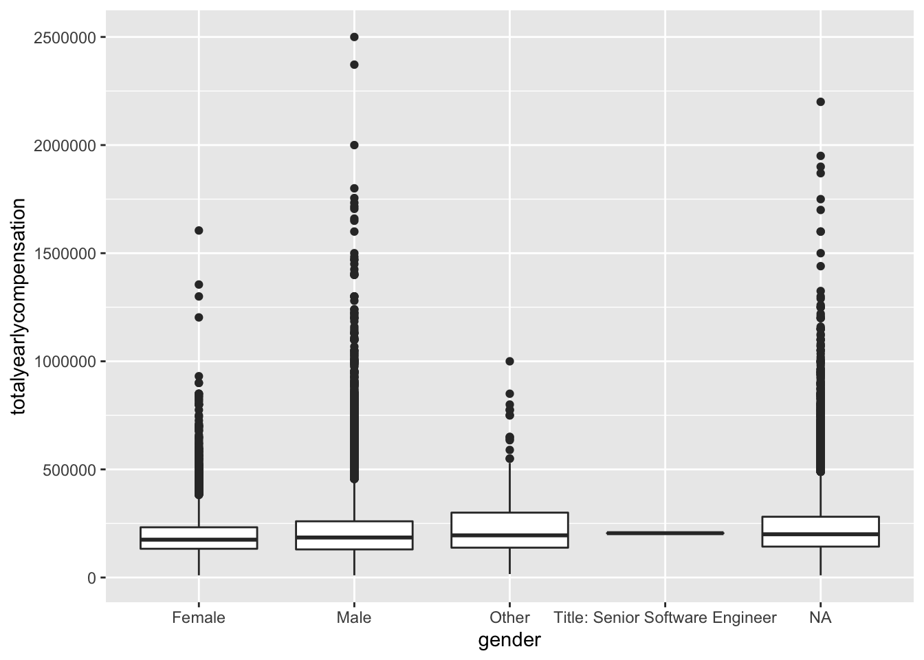
salary%>% arrange(desc(totalyearlycompensation)) %>% filter(totalyearlycompensation < 3000000) %>% ggplot(aes(x = Race, y = totalyearlycompensation)) + geom_boxplot()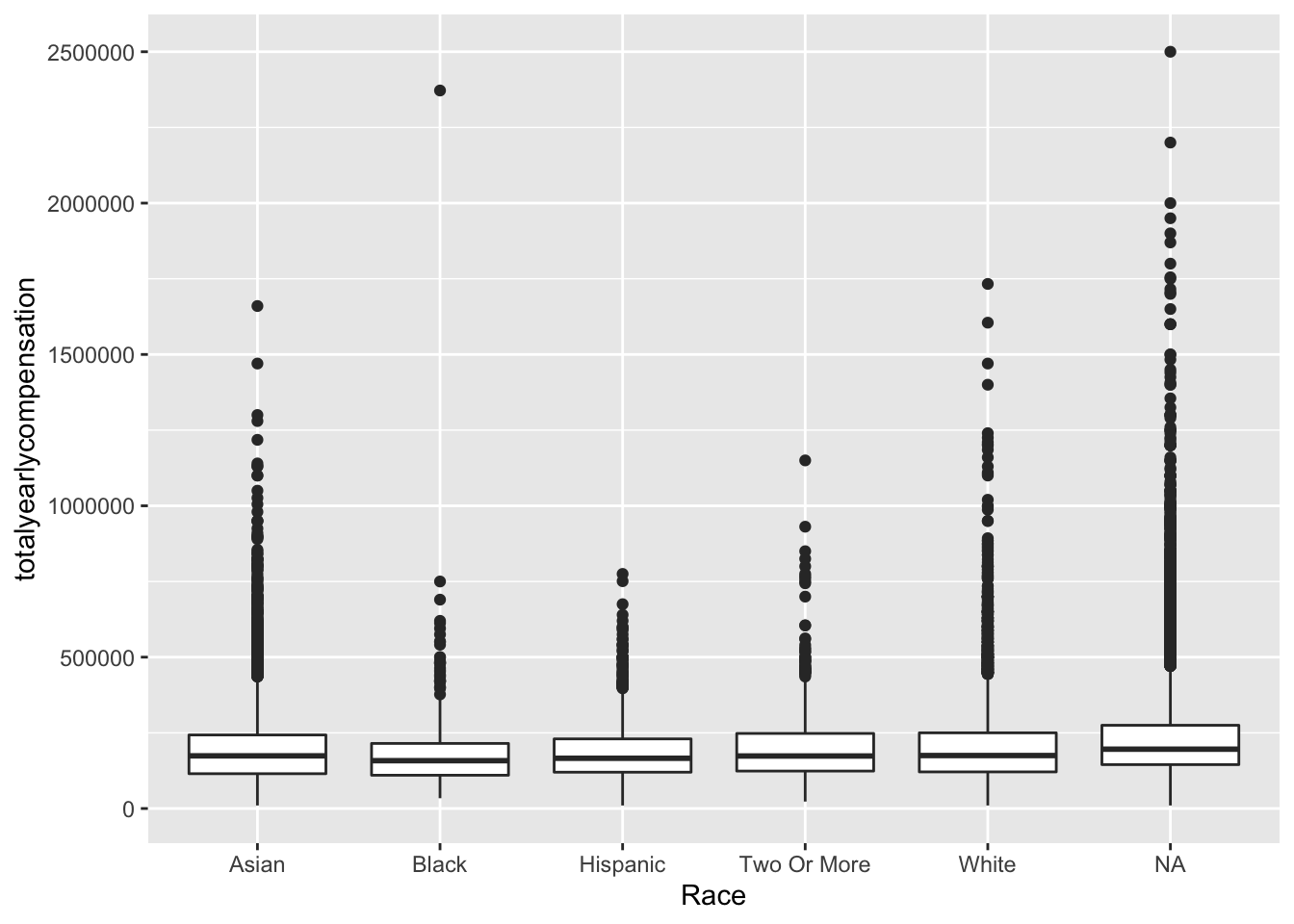
salary %>% arrange(desc(totalyearlycompensation)) %>% filter(totalyearlycompensation < 3000000)%>% ggplot(aes(x = Education, y = totalyearlycompensation)) + geom_boxplot()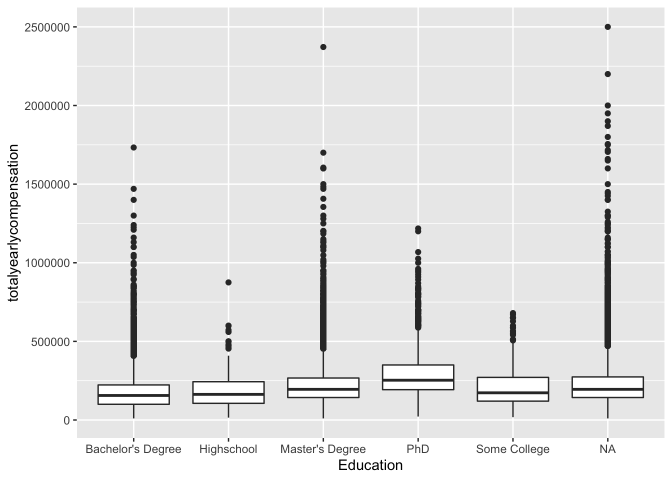
salary %>% arrange(desc(totalyearlycompensation)) %>% filter(totalyearlycompensation < 3000000)%>% ggplot(aes(x = yearsofexperience, y = yearsatcompany)) + geom_smooth()## `geom_smooth()` using method = 'gam' and formula 'y ~ s(x, bs = "cs")'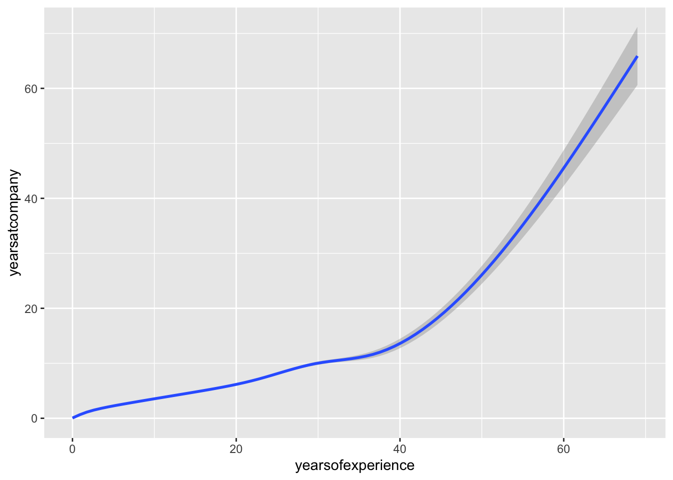 What are the big, obvious patterns in the data? Are these surprising?
## no big difference between NA and other categories in these three variables, and we observed a strong correlation between years of experience and years at company, the correlation need to be addressed…,,,,,
What are the big, obvious patterns in the data? Are these surprising?
## no big difference between NA and other categories in these three variables, and we observed a strong correlation between years of experience and years at company, the correlation need to be addressed…,,,,,