
\[\\[0.2in]\]
Exploratory Analysis and Modeling
\[\\[0.2in]\] Motivated by our big picture page, we are shocked by how destructive unregulated mortgage issuance can be to the US economy or even the world. In 2010, the US government promulgated the Dodd Frank Act, which aims to strengthen the risk control and supervision on the entire financial market. Among the act, the monitoring of the mortgage market is the top priority. How to ensure that loan funds flow into the pockets of those who can repay is now a flag for the mortgage industry. The introduction of credit risk control in the mortgage market is not only in line with the new policy, but also has a very promising future. Therefore, we would like to combine what we learnt from data science to measure the credit risk of mortgage default. \[\\[0.2in]\]
Meanwhile, we found that the subprime mortgage crisis did not happen overnight. Before the crisis, there have been many signs that the housing loan market has been overheating, such as the oversupply in housing market, a short-term increase in housing loan interest rates, a decline in average credit scores, and a bubble in the real estate industry. We are sure that these market phenomena and indexes have a strong relationship with the mortgage default rate. Some are positively correlated, such as mortgage interest rates. Some are negatively correlated, such as individual credit scores. Motivated by these patterns, we would like to uncover the relationship between default probability and different variables including macroeconomic and personal data of specific loans in our EDA. After that, we will conduct a feature selection to filter out useful variables and fit them into different models. \[\\[0.2in]\]
With that said, there are certain conflicts and limitations in our research. We believe that more variable about personal information can definitely help us determine default probability of specific mortgages. However, we are also worried that acquiring too much personal data may infringe privacy of others. We hope that our model can be accurate without abusing personal information, and we believe that this is one of the most critical ethics problem for most data scientists. Therefore, we hope that we can achieve a balance between accuracy and privacy. \[\\[0.2in]\]
As we discussed before, the collapse of financial derivative of mortgage like back securities is also a trigger for mortgage default in 2008. From our perspective, stock index can be a good indicator to measure the risk of these financial products. Therefore, to better measure the influence of financial market to mortgage default rate, we combined our S&P stock market index with our major data set to create a new variable: Mean S&P Stock Market Index. Below is the variables that we are interested, and we would like to determine their relationships with default or not one by one. \[\\[0.2in]\]
| Column Name | Description |
|---|---|
| orig_time | Time stamp for origination of the mortgage |
| REtype_SF_orig_time | Single family home |
| investor_orig_time | With investor |
| balance_orig_time | Outstanding balance at origination time |
| FICO_orig_time | FICO credit score |
| LTV_orig_time | Initial loan to value ratio |
| state_orig_time | US state in which the property is located |
| hpi_orig_time | House price index at the origination of the mortgage, base year=100 |
| age | number of periods from origination of the mortgage to its end |
| interest_rate_mean | the average interest rate of all observation periods |
| gdp_mean | the average GDP growth of all observation periods |
| uer_mean | the average unemployment rate of all observation periods |
| default_time | Default Status |
| SP | Mean S&P Stock Index during all observation period |
\[\\[0.2in]\]
To confirm our directions, we would like to first make a correlation map between default and different explanatory variables: \[\\[0.2in]\]
# Code from: http://www.sthda.com/english/wiki/ggplot2-quick-correlation-matrix-heatmap-r-software-and-data-visualization
mydata <- mortgage_norm %>% select(default_time,orig_time, REtype_SF_orig_time,investor_orig_time, balance_orig_time,FICO_orig_time, LTV_orig_time, interest_rate_mean, hpi_orig_time,TTM,uer_mean,gdp_mean,age,SP)
names(mydata) = c('Default or Not','Original Time', 'Single Family', 'With Investor', 'Original Balance','FICO Credit Score','Loan to Value','Interest Rate', 'House Price Index', 'Time to Maturity','Unemployment Rate','GDP Growth','Age','S&P Stock Index')
cormat <- round(cor(mydata),2)
get_upper_tri <- function(cormat){
cormat[lower.tri(cormat)]<- NA
return(cormat)
}
upper_tri <- get_upper_tri(cormat)
melted_cormat <- melt(upper_tri, na.rm = TRUE)
reorder_cormat <- function(cormat){
dd <- as.dist((1-cormat)/2)
hc <- hclust(dd)
cormat <-cormat[hc$order, hc$order]
}
cormat <- reorder_cormat(cormat)
upper_tri <- get_upper_tri(cormat)
melted_cormat <- melt(upper_tri, na.rm = TRUE)
ggheatmap <- ggplot(melted_cormat, aes(Var2, Var1, fill = value))+
geom_tile(color = "white")+
scale_fill_gradient2(low = "steelblue4", high = "skyblue", mid = "white",
midpoint = 0, limit = c(-1,1), space = "Lab",
name="Pearson\nCorrelation Map") +
theme_minimal()+ theme(axis.text.x = element_text(angle = 45, vjust = 1,
size = 9, hjust = 1)) + coord_fixed()
ggheatmap +
geom_text(aes(Var2, Var1, label = value), color = "black", size = 2.3) +
theme(
axis.title.x = element_blank(),
axis.title.y = element_blank(),
panel.grid.major = element_blank(),
panel.border = element_blank(),
panel.background = element_blank(),
axis.ticks = element_blank(),
legend.justification = c(1, 0),
legend.position = c(0.6, 0.7),
legend.direction = "horizontal") +
guides(fill = guide_colorbar(barwidth = 7, barheight = 1,
title.position = "top", title.hjust = 0.1))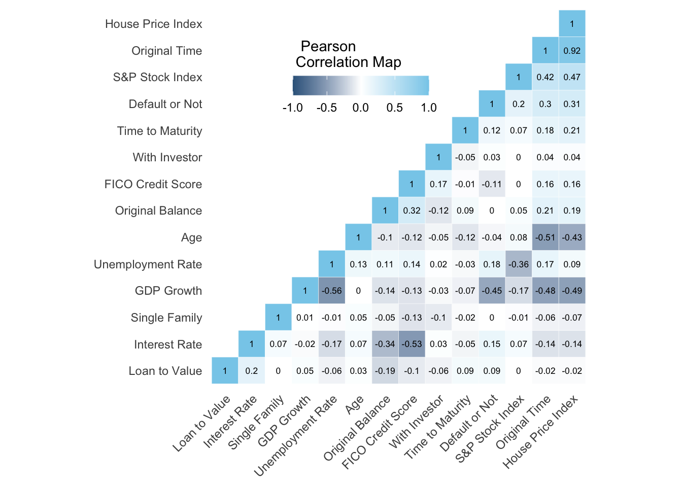 \[\\[0.2in]\]
The Pearson Correlation map above shows the correlations among all variables we have in the time frame of 2000 and 2014. In this map, blue indicates positive relationships and grey indicates negative relationships. We find out that GDP growth has the strongest negative correlations with default or not, which is -0.45. That means that as GDP growth goes higher, the probability of default goes lower. The situation is similar for interest rate and GDP growth with a negative correlation of -0.15. What is more, FICO score which indicates one’s credit is also proven to be important with a correlation of -0.11. As we expected, unemployment rate are the only economic data positively correlated to default probability.
\[\\[0.2in]\]
We also found out that there are a few strong negative correlations between several different variables, which includes Interest Rate vs. FICO Credit Score, Default or not vs. GDP growth, original time vs. GDP growth, House price index vs. GDP growth, Age vs. Original time, and Age vs. House price index. Therefore, we believe that a feature selection process will be important to eliminate pairwise influence and omitted variable bias. Outside economy and inside personal information will both be our focus, and we also hope to measure the difference of their influence to mortgage default probability. As followed, we will start to uncover the relationship between these variables and default probability: \[\\[0.2in]\]
Default Probability vs. GDP Growth:
\[\\[0.2in]\]
mortgage_norm %>% filter(status_last!= 0) %>% mutate(status = ifelse(default_time == 1, 'Default','Payoff')) %>%ggplot(aes(x=gdp_mean, fill= status))+ geom_density(alpha=.5,colour = 'white')+ geom_vline( xintercept= 2.305184, linetype="dashed", size=.7, colour = 'steelblue1') + theme_bw()+geom_vline( xintercept= 1.172898 , linetype="dashed", size=.7, colour = 'steelblue4') + scale_fill_manual(name = 'Distribution',values=c("steelblue4", "steelblue1")) + labs(x = "GDP Growth", y = 'Density', title = 'Mortgages Distribution Map According to GDP Growth',subtitle = 'Dashed Line: Mean GDP Growth') + theme(plot.title = element_text(face="bold",size = 15))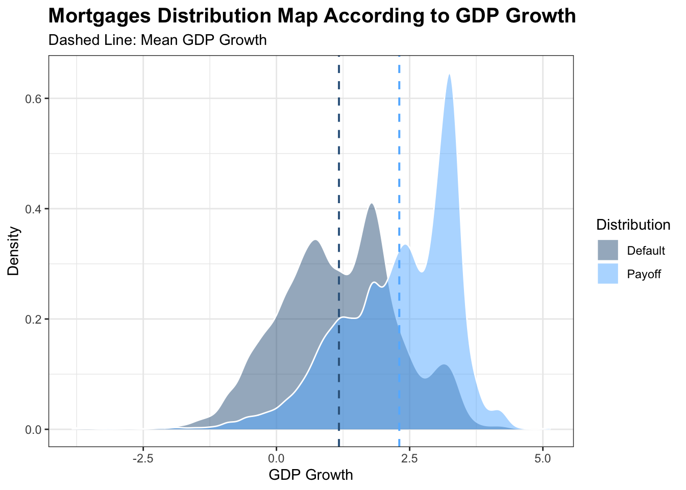
\[\\[0.2in]\]
The map of mortgages distribution shows us the relationship between the density of mortgages in both default and payoff and GDP growth between 2000 and 2014. As we can see that, both status are mainly in normal distribution. The grey map represents distribution of default mortgages in different GDP growth and the blue map measures those payoffs. The dash lines show us that the mean GDP growth of mortgages in default is smaller than the one with mortgages in payoff. We can see that the shape of distribution are very similar for both Defaults and Payoffs. However, if we take GDP growth into account, it is evident that most default mortgages mainly resides in where GDP growth is lower, which is totally on the left of those payoffs. In that case, we are confident that as GDP growth goes higher, default probability are more likely to be lower, and Vice Versa.
\[\\[0.2in]\]
Default Probability vs. Origination Time:
\[\\[0.2in]\]
a <- mortgage_norm %>% separate(first_time_date, into = c('year','month','date'),sep ='-') %>% group_by(year,default_time) %>% summarise(n = n()) %>% pivot_wider(names_from = 'default_time',values_from = 'n') ## `summarise()` has grouped output by 'year'. You can override using the `.groups` argument.a[is.na(a)] <- 0
names(a) = c('Time','Payoffs','Defaults')
a %>% mutate(Total = Defaults + Payoffs, Default_Portion = Defaults/Total) %>% ggplot() + geom_line(aes(x = Time, y = Default_Portion),color = 'steelblue3',group = 1) + geom_point(aes(x = Time, y = Default_Portion,size = Total),color = 'steelblue3')+ theme_bw() + scale_size_continuous(breaks = c(1500,3000,6000,12000)) + labs(x = "Start Time", y = 'Default Portion', title = 'Default Mortgages Portions According to Their Start Time', size = ' Total Mortgages') + theme(plot.title = element_text(face="bold",size = 14))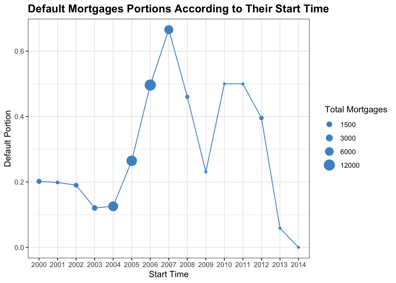
\[\\[0.2in]\]
The plot shows us default mortgages portions according to their start time from 2000 to 2014 and the number of mortgages each year. According to the graph, during 2004 to 2007, the number of total mortgages were much larger compared to the rest of years, which were roughly 6000 to 12000, and the default portions increased dramatically in these years from about 0.2 to 0.7. However, right after 2007, we see a big drop in the number of mortgages and mortgages in default. And after a rise during 2009 and 2011, the number of mortgages stays relatively the same and small, but the portion of mortgages in default decreases in remarkably and even down to 0 in 2014. We believe that the difference is because of economic crisis and government regulations right after that. The release of the Dodd Frank act strongly regulates mortgage market. Therefore, the number of mortgage and default rate decreases dramatically after 2010, which fits perfectly to the release time of the act. However, the influence of origination time to default probability can be somewhat represented the GDP growth. Therefore, this variable might be useless to measure default.
\[\\[0.2in]\]
Default Probability vs. SingleFamily:
\[\\[0.2in]\]
mortgage_norm %>% count(default_time, REtype_SF_orig_time) %>% mutate(SF = ifelse(REtype_SF_orig_time == 1, 'SingleFamily','Non_SingleFamily')) %>% mutate(Default = ifelse(default_time == 1, 'Default','Payoff'))%>% ggplot(aes(x= factor(SF), y = n, fill= factor(Default))) + geom_bar(position = 'dodge', stat='identity') + geom_text(aes(label= n), color = 'white',size = 4, position = position_dodge(width=0.9), vjust=5, fontface = 'bold')+ theme_bw() + labs(x = '', y = 'Total Number', title = 'Compare Default or Not and Single Family Status',fill = 'Mortgage Status')+ theme(plot.title = element_text(face="bold",size = 15))+ scale_fill_manual(values = c('steelblue4','steelblue2'))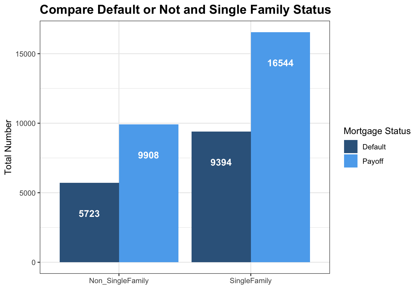
\[\\[0.2in]\]
The bar chart here shows the number of mortgages in default and payoff comparing non-single family and single family in the time frame of 2000 and 2014. By directly comparing the two bar graphs, it seems that single family tends to have a higher number of defaults. However, we can see that a larger portion of mortgages in our dataset are single family. Therefore, to compare the default/payoff ratio between each graph is more meaningful for us. However, there is no much difference just by first glance.
\[\\[0.2in]\]
Default Probability vs. Investor Status:
\[\\[0.2in]\]
mortgage_norm %>% count(default_time, investor_orig_time) %>% mutate(SF = ifelse(investor_orig_time == 1, 'With Investor','Without Investor')) %>% mutate(Default = ifelse(default_time == 1, 'Default','Payoff'))%>% ggplot(aes(x= factor(SF), y = n, fill= factor(Default))) + geom_bar(position = 'dodge', stat='identity') + geom_text(aes(label= n), color = 'white',size = 3.5, position = position_dodge(width=0.9), vjust=1.6,fontface = 'bold')+ theme_bw() + labs(x = '', y = 'Total Number', title = 'Compare Default or Not and Investor Status',fill = 'Mortgage Status')+ theme(plot.title = element_text(face="bold",size = 15))+ scale_fill_manual(values = c('steelblue4','steelblue2'))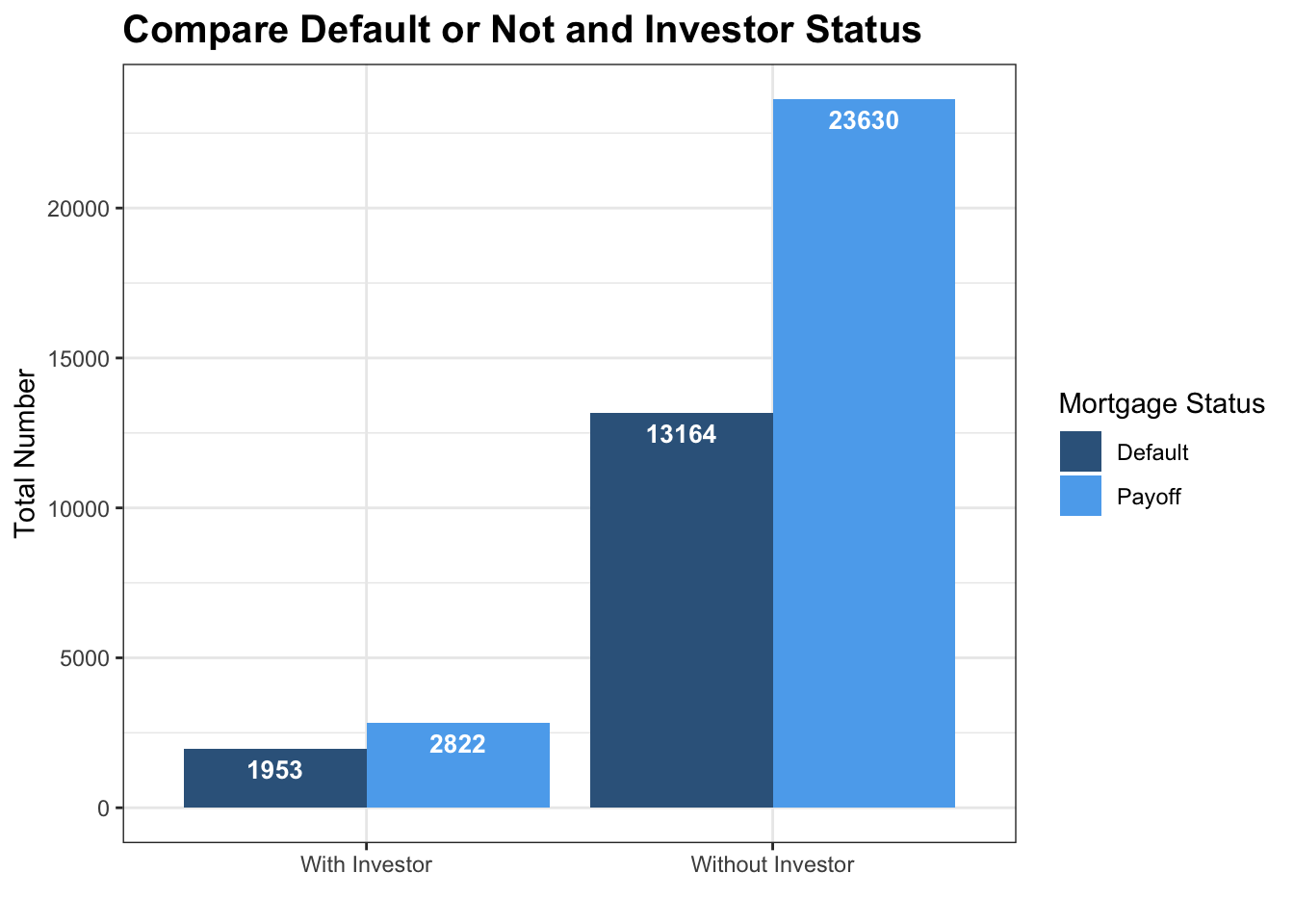
\[\\[0.2in]\]
This bar graph shows the number of mortgages separated by default status and with investor or not. According to the graph, it shows an obvious difference between the number of mortgages with investor and without investor. The number of mortgages without investor is significantly higher than the number of mortgages with investor. Moreover, it is shown in the graph that mortgages with investors tends to have a much higher ratio of default. This totally contradicts our assumption, because we think that individual investors will be more informed to determine the default probability of specific mortgages. However, the answer turns out to be not, therefore, we now tend to believe that most investors hoping for higher return tends to select mortgage with higher interest rate, which is subject to higher risk of defaults. So we make another plot to determine the difference of interest rate with and without investors.
\[\\[0.2in]\]
mortgage_norm %>% group_by(investor_orig_time) %>% summarise(a = mean(interest_rate_mean)) %>% mutate(SF = ifelse(investor_orig_time == 1, 'With Investor','Without Investor')) %>% ggplot(aes(x = SF, y = a, fill = SF)) + geom_col() + coord_cartesian(ylim = c(7, 8))+theme_bw()+theme(plot.title = element_text(face="bold",size = 15))+ labs(y = 'Interest Rate',title = 'Compare Interest Rate and Investor Status', fill = 'Single Family Status')+scale_fill_manual(values = c('steelblue4','steelblue2'))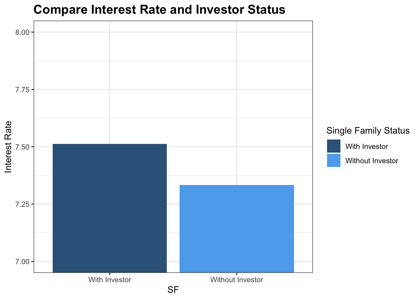
\[\\[0.2in]\]
As we can see from the chart that mortgage with investors tends to have a much higher interest rate for a higher return. In that case, they might experience a greater risk of mortgage default.
\[\\[0.2in]\]
Default Probability vs. Mortgage Size:
\[\\[0.2in]\]
mortgage_norm %>% mutate(Default = ifelse(default_time == 1, 'Default','Payoff')) %>% filter(balance_orig_time <= 650000) %>% ggplot() + geom_boxplot(aes(x = factor(Default), y = balance_orig_time, fill = factor(Default)),size = 0.5, color = 'grey40') + theme_bw()+ scale_fill_manual(values = c('steelblue4','steelblue2')) + labs(y = 'Mortgage Size', x = '', title = 'Compare Default Status and Mortgage Size', fill = 'Mortgage Status')+ theme(plot.title = element_text(face="bold",size = 15))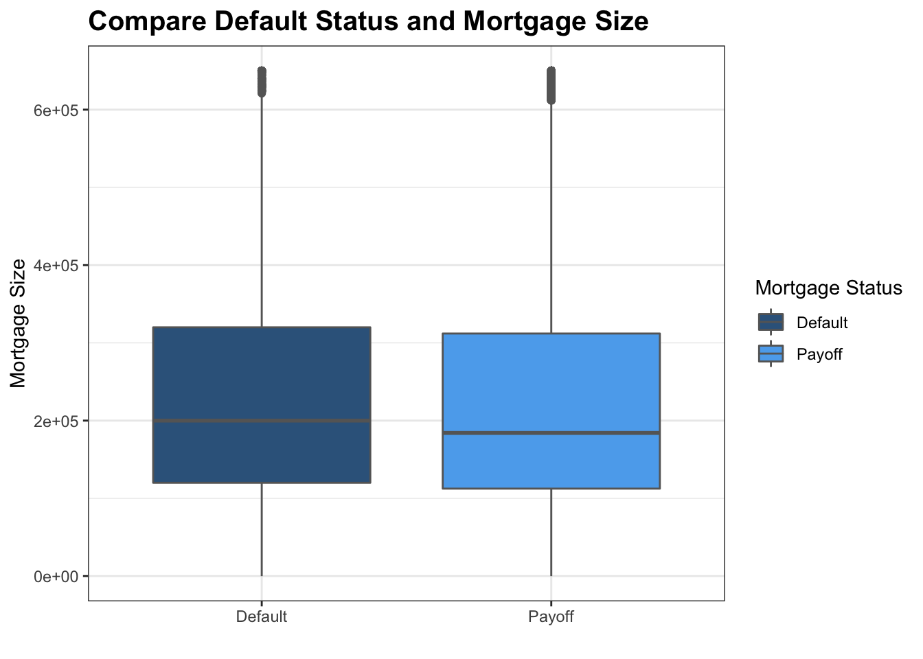
\[\\[0.2in]\]
This boxplot shows the relationship between the mortgage size and the mortgage status. Since there are a few outsiders with extremely large size, we filter out mortgages that are larger than 650000 dollars to avoid distortion of the view. It is shown in the graph that the medium of the mortgage size in default status and payoff status are very close, and the ranges are roughly the same between default and payoff. With that said, the 25th percentile, medium, and 75th percentile tends to be larger for default mortgages. We believe that maybe that is because the more expensive a mortgage is, the harder for people to payoff its loan. However, this is just a guess without evidence. However, as we focus on mortgage that are around 650000 dollars, there are more payoff compare to defaults, is it because the rich has a better ability to pay? More data are needed to figure this out.
\[\\[0.2in]\]
###Default Probability vs. FICO Credit Score: \[\\[0.2in]\]
mortgage_norm %>% count(default_time)## # A tibble: 2 x 2
## default_time n
## <dbl> <int>
## 1 0 26452
## 2 1 15117mortgage_norm %>% summarise(meanc = mean(FICO_orig_time))## # A tibble: 1 x 1
## meanc
## <dbl>
## 1 660.mortgage_norm %>% filter(FICO_orig_time >= 450) %>% mutate(Default = ifelse(default_time == 1, 'Default','Payoff')) %>% ggplot() + geom_density(aes(x = FICO_orig_time, fill = factor(Default)), position = 'fill',color = 'white',alpha = 0.85)+ theme_bw()+ scale_fill_manual(values = c('steelblue4','steelblue2')) + annotate('text',x = 550, y = 0.75,label = 'Total Defaults: 15117',color = 'white') + annotate('text',x = 750, y = 0.25,label = 'Total Payoffs: 26452 ',color = 'white') + labs(x = 'FICO Credit Score', y = 'Density', title = 'FICO Credit Score Density Map by Default Status',subtitle = 'Dashed Line: Mean FICO Credit Score', fill = 'Mortgage Status')+geom_vline(xintercept= 659.7322, linetype="dashed", size=.7, colour = 'steelblue4', alpha =0.8)+ theme(plot.title = element_text(face="bold",size = 13)) 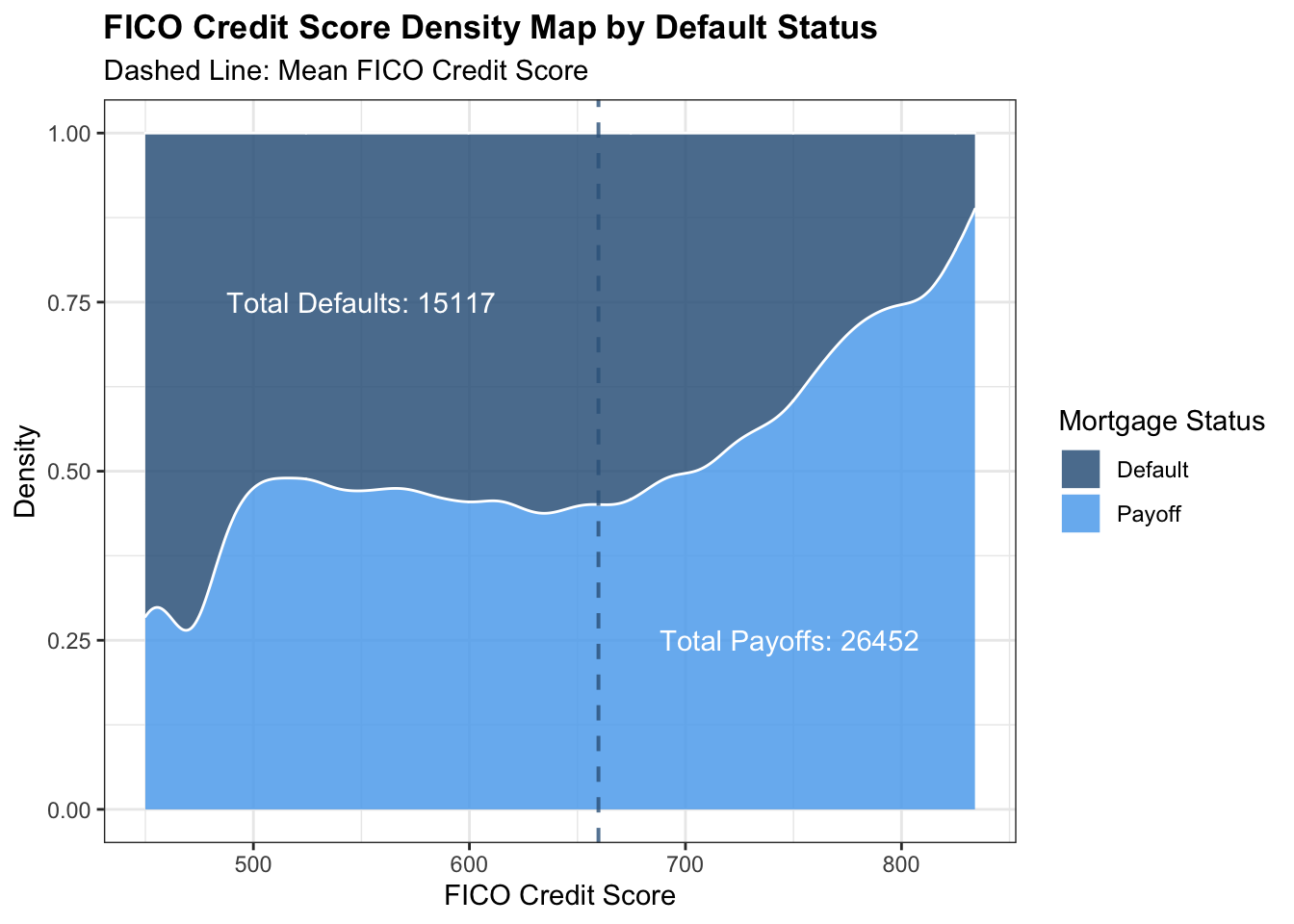
\[\\[0.2in]\]
FICO scores are one kind of credit score.The name derives from the Fair Isaac Corp., which introduced the FICO score in 1989. The terms “credit score” and “FICO score” are often used interchangeably, but there are other brands of scores. FICO score is one of the most important variable that we would like to use to measure default probability. This graph shows us the relationship between the ratio of default and payoff mortgages and the FICO credit score. According to the graph, it is shown that the portion of default mortgages decreases as the FICO credit score increases.So there is a negative correlation between the FICO credit score and default probability as indicated by the correlation map. When, credit score are lower to about 400, about 75% of people will default. However, as the credit score goes up to about 850, only less than 10% of people will default. When in mean credit score, the default probability is about 50%. We believe that FICO score are strongly correlated to one’s ability to pay back, which should be concerned by banks when considering making mortgages.
\[\\[0.2in]\]
###Default Probability vs. Interest Rate:
\[\\[0.2in]\]
a <- mortgage_norm %>% separate(last_time_date, into = c('year','month','date'),sep ='-') %>% count(year, default_time) %>% pivot_wider(names_from = 'default_time', values_from = 'n')
b <- mortgage_norm %>% separate(last_time_date, into = c('year','month','date'),sep ='-') %>% group_by(year) %>% summarise(meaninterest = mean(interest_rate_mean), Total = n()) %>% left_join(a, by = 'year')
names(b) = c('year', 'Interest_Rate','Total','Payoffs','Defaults')
b <- b %>% mutate(default_portion = Defaults/Total)
b %>% ggplot(aes(x = year, y = Interest_Rate)) + geom_line(group = 1, color = 'steelblue4') + geom_point(aes(size = Total, color = default_portion)) + theme_bw() + labs(x = 'Year',y = 'Interest Rate', size = 'Total Mortgages',color = 'Default Portion', title = 'Portion of Mortgages Ended in Default as Interest Rate Changing') + scale_color_gradient(low = 'skyblue1', high = 'dodgerblue4')+theme(plot.title = element_text(face="bold",size = 12)) 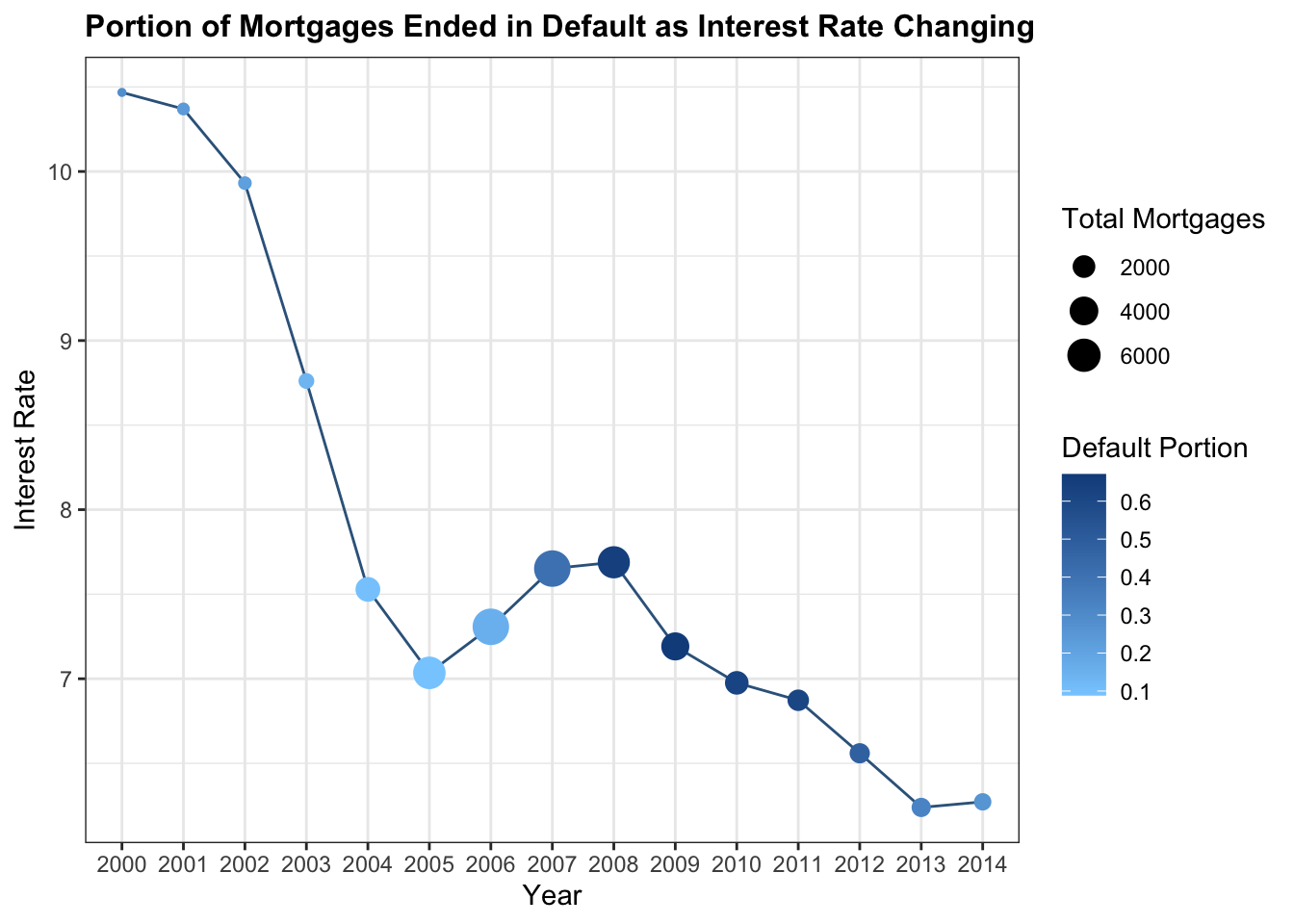
\[\\[0.2in]\]
Interest rate is one of the most important variables to be focused in our EDA. As we mentioned before, a lot of mortgage during the economic crisis are with adjustable interest rate. Therefore, as the interest rate goes higher, the general public’s ability to payback also goes lower. This graph shows the relationship between interest rate changes and the portion of mortgages ended in default status. According to the graph, from 2000 to 2005, interest rate decreases dramatically from about 11 to 7. The total number of mortgages are also increasing in this period, since it is cheaper for people to buy a house. The default portion also remains steady by this period. However, between 2005 and 2008, there is a significant increase from 7 to about 7.8, which is partly because of government’s intention to cool the housing market.By this time, the default portion of mortgage rises dramatically from 0.1 to 0.7, which is terrific. This is also the time with most number of mortgages. Therefore, the influence of interest rate cannot be ignored when measuring one’s ability to payback the loan. After strengthening regulation on mortgage market, we can see that the default portion starts to decrease.
\[\\[0.2in]\]
###Default Probability vs. unemployment Rate:
\[\\[0.2in]\]
mortgage_norm %>% ggplot(aes(x=uer_mean,fill= factor(default_time)))+ geom_histogram(aes(fill= factor(default_time)), color = 'white', position='identity',binwidth = 0.2) + theme_bw()+ scale_fill_manual(name = 'Mortgage Status',values = c('steelblue4','steelblue2'),labels = c('Payoff','Default')) + labs(x = 'Unemployment Rate', y = 'Total Mortgages',title = 'Compare Default Portion and Unemployment Rate')+ theme(plot.title = element_text(face="bold",size = 13)) 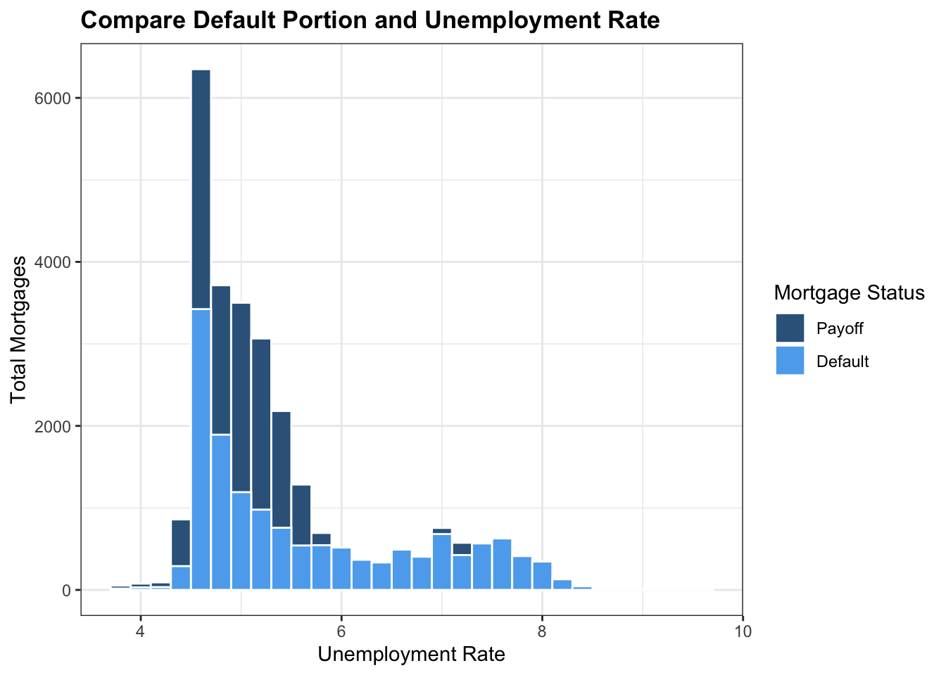
\[\\[0.2in]\]
This histogram here shows us the relationship between the number of default and payoff mortgages and the mean unemployment rate. According to this graph, it is apparent that the most mortgages experience a mean unemployment rate of about 4 to 6, which has a default/payoff ratio of about 0.5. However, after the unemployment rate passes 6, the total number of mortgages drops significantly, but the portion of default increases dramatically as almost all mortgages are in default. Therefore, it is evident that as the unemployment rate goes higher, people’s ability to pay the mortgage goes lower. When the unemployment rate is higher than 6%, default probability of most mortgages is almost 100%. This is reasonable, because as people lose their job, they are unable to payback their mortgages also.
\[\\[0.1in]\]
###Default Probability vs. Loan to Value Ratio:
\[\\[0.2in]\]
mortgage_norm[sample(nrow(mortgage_norm ), 20000),] %>% filter(LTV_orig_time <= 110) %>% mutate(Default = ifelse(default_time == 1, 'Default','Payoff')) %>% ggplot()+ geom_point(aes(x = factor(Default), y = LTV_orig_time, color = factor(Default)), position = 'jitter',size = 0.5, alpha = 0.3) + theme_bw()+scale_color_manual(values = c('steelblue4','steelblue2')) + annotate('text', x = 1, y = 105, label = 'Total: 15117', color = 'steelblue4', fontface = 'bold', size = 5) + annotate('text', x = 2, y = 105, label = 'Total: 26452', color = 'steelblue2', fontface = 'bold', size = 5) + labs(color = 'Mortgage Status',x = '', y = 'Original Loan to Value', title = 'Compare Original Loan to Value with Default Status')+theme(plot.title = element_text(face="bold",size = 13)) 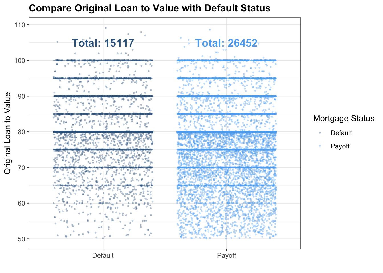 \[\\[0.2in]\]
This is a plot between default status and loan to value ratio. To make the scatter plot more visible, we randomly select 20000 mortgages in our dataset, which is about half of the total mortgages. In both default and payoff status, there is a clear segregation at the point where original Loan to Value is 80: the density of points at Original Loan to Value = 80 is the highest, which makes the line there looks thicker than all other lines. Also, the points below Original Loan to Value = 80 is clearly more than points that are above this point, indicating that in both default and payoff status, the majority’s Original Loan to Value is below 80. However, one thing worth noticing is that in ratio less than 0.7, there are much more payoff compare to defaults. In that case, we believe that people with a lower Loan to Value ratio are more likely to payback their mortgages.
\[\\[0.2in]\]
Default Probability vs. Age:
\[\\[0.2in]\]
b <- mortgage_norm %>% count(age,default_time) %>% pivot_wider(values_from = 'n', names_from = 'default_time')
names(b) = c('age','payoff','default')
b[is.na(b)] <- 0
b <- b %>% mutate(total = default + payoff, default_portion = default/total ) %>% filter(age <= 39)
b$year <- rep(1:10,each = 4)
b %>% group_by(year) %>% summarise(Default_Portion = mean(default_portion), SD = sd(default_portion),Total = mean(total)) %>% filter(year <= 13) %>% ggplot(aes(x=year, y=Default_Portion)) + geom_line(color = 'steelblue4') + geom_point(aes(size = Total),color = 'steelblue4') + geom_errorbar(aes(ymin=Default_Portion-SD, ymax=Default_Portion+SD), width=.2, position=position_dodge(0.05),color = 'steelblue4') + theme_bw() + labs(y = 'Default Portion', x = 'Age', size = 'Total Mortgages', title = 'How Default Portion Changes with Age of Mortgages') + theme(plot.title = element_text(face="bold",size = 13))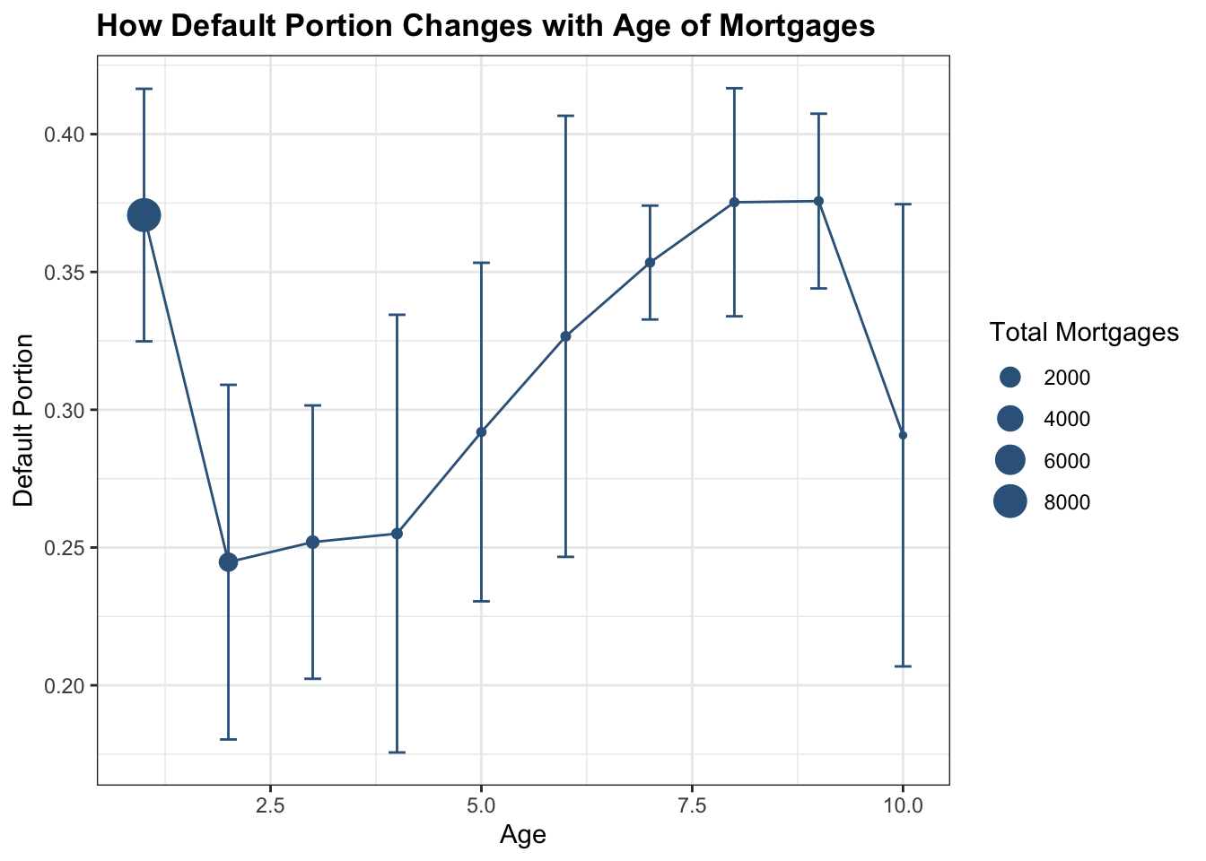
\[\\[0.2in]\]
We use error bar here to show how default probability floats with mortgage’s age. As the graph shows, default portion has the highest level when the age of mortgage is around 1.25 years or between 7.5 and 8.75 years, which is around 0.375. When the mortgage age is between 2.5 and 3.75 years, default portion is stable around 0.25; and then the default portion raise up to its highest level from age of 3.75 years to 7.5 years; then the portion fall back down to below 0.3 when the mortgage age approaches 10 years. The error bar goes larger as the age goes higher, we believe that is because there are less observations. However, we believe that the reason why most mortgages default in year 1 is because that most of them are originated right before the global financial crisis. They default right after the collapse of the economy. In that case, this variable may be biased.
\[\\[0.2in]\]
###Default Probability vs. House Price Index:
mortgage_norm %>% ggplot(aes(x=hpi_orig_time,fill= factor(default_time)))+ geom_histogram(aes(fill= factor(default_time)), color = 'white', position='identity',binwidth = 5) + theme_bw()+ scale_fill_manual(name = 'Mortgage Status',values = c('steelblue4','steelblue2'),labels = c('Payoff','Default')) + labs(x = 'House Price Index', y = 'Total Mortgages',title = 'Compare Default Portion and House Price Index')+ theme(plot.title = element_text(face="bold",size = 13)) 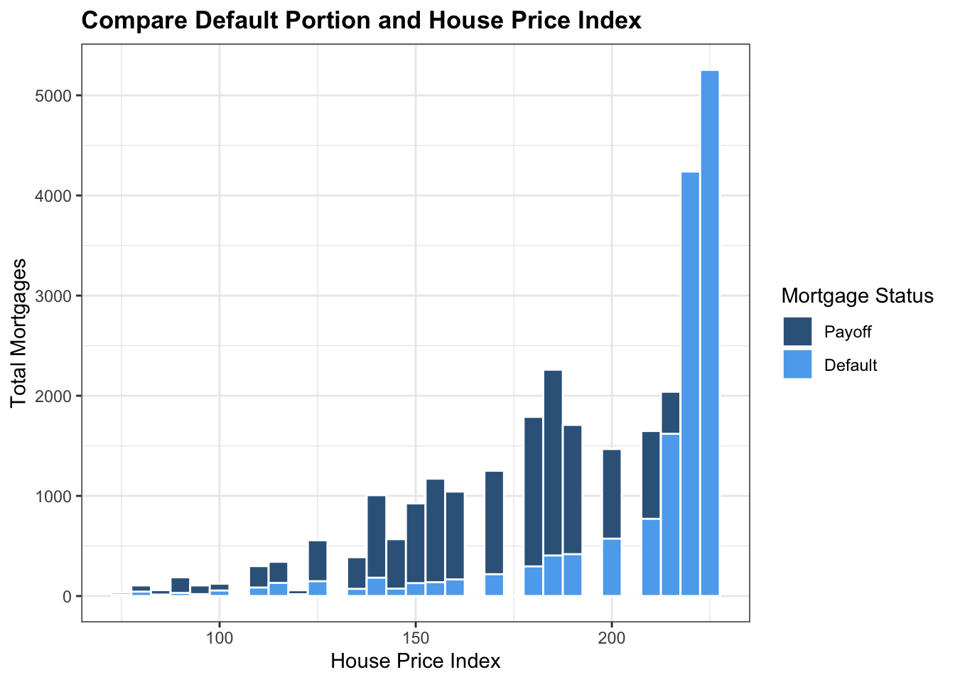 \[\\[0.2in]\]
We choose the initial house price index to compare with default status, because we assume no refinance of mortgages in our dataset. As the graph shows, when the House Price Index is less than 200, payoff status outnumbered default status in all situations. But when House Price Index is more than 200, portion of default increased drastically and outnumbered payoff portion; and finally, the default rate becomes 100% as the House Price Index increases to more than 200. This is obvious that as the price of the house goes higher, people are less likely to pay back their loans.
\[\\[0.2in]\]
a <- mortgage_norm %>% separate(last_time_date, into = c('year','month','date'),sep ='-') %>% count(year, default_time) %>% pivot_wider(names_from = 'default_time', values_from = 'n')
b <- mortgage_norm %>% separate(last_time_date, into = c('year','month','date'),sep ='-') %>% group_by(year) %>% summarise(meanSP = mean(SP), Total = n()) %>% left_join(a, by = 'year')
names(b) = c('year', 'SP_Index','Total','Payoffs','Defaults')
b <- b %>% mutate(default_portion = Defaults/Total)
b %>% ggplot(aes(x = year, y = SP_Index)) + geom_line(group = 1, color = 'steelblue4') + geom_point(aes(size = Total, color = default_portion)) + theme_bw() + labs(x = 'Year',y = 'S&P Stock Market Index', size = 'Total Mortgages',color = 'Default Portion', title = 'Portion of Mortgages Ended in Default as Stock Market Index Changing') + scale_color_gradient(low = 'skyblue1', high = 'dodgerblue4')+theme(plot.title = element_text(face="bold",size = 11)) 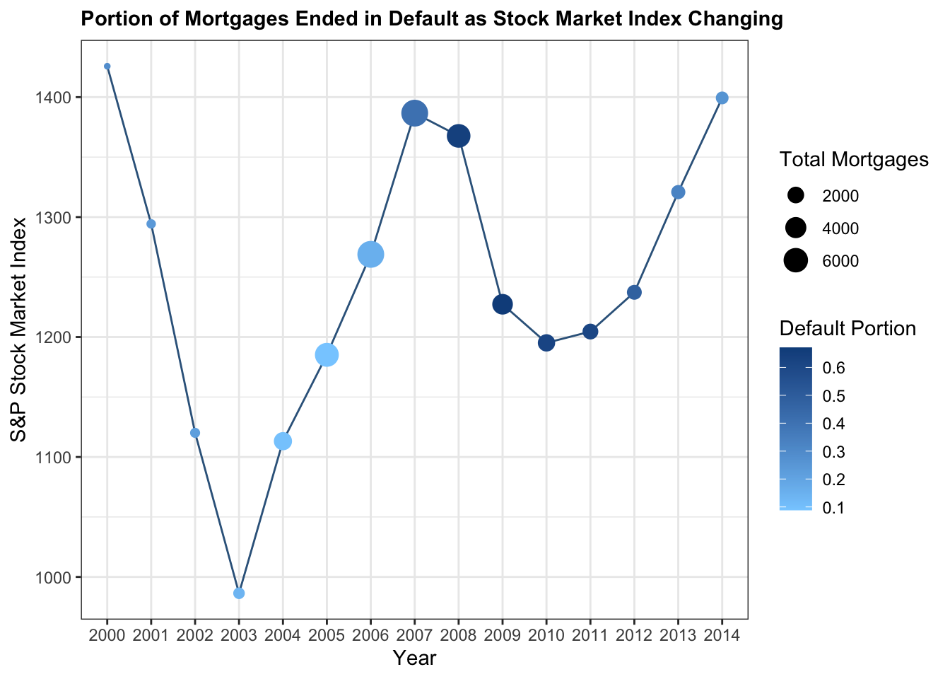
As the graph shows, before the year of 2007, though the Stock Market Index changed drastically – a sharp decrease from 1450 in year 2000 to below 1000 in year 2003, and then a sharp increase to 1400 in year 2007 – the default portion during these years didn’t change a lot, which is always around 10%. However, in year 2008, as the global economic crisis happened, the default portion has increased to over 60% until year 2013. This is reasonable because by 2003 to 2007, a huge amount of financial derivative of mortgage released. In that case, financial market started to link mortgage default probability. As the stock index dropped from 1400 to around 1200, mortgage default portion rises in unprecedented speed. Therefore, financial market status should be considered when marking loan to house buyer.
\[\\[0.2in]\]
Default Probability vs.State:
\[\\[0.2in]\]
mortgage_last<-mortgage %>% group_by(id) %>%  summarise_all(last)
epsg_us_equal_area <- 2163
us_states <- st_read(here::here("dataset/cb_2019_us_state_20m/cb_2019_us_state_20m.shp"))%>%
  st_transform(epsg_us_equal_area)
## Reading layer `cb_2019_us_state_20m' from data source
## `/Users/alex/Desktop/fa2021-final-project-digfora/dataset/cb_2019_us_state_20m/cb_2019_us_state_20m.shp'
## using driver `ESRI Shapefile'
## Simple feature collection with 52 features and 9 fields
## Geometry type: MULTIPOLYGON
## Dimension: XY
## Bounding box: xmin: -179.1743 ymin: 17.91377 xmax: 179.7739 ymax: 71.35256
## Geodetic CRS: NAD83not_contiguous <-
c("Guam", "Commonwealth of the Northern Mariana Islands",
"American Samoa", "Puerto Rico", "Alaska", "Hawaii",
"United States Virgin Islands")
us_cont <- us_states %>%
filter(!NAME %in% not_contiguous) %>% filter(NAME != "District of Columbia") %>%
transmute(STUSPS,STATEFP,NAME, geometry)
p <- mortgage %>% group_by(state_orig_time) %>% summarize(count = n(),def = sum(status_time[status_time == 1])) %>% mutate(proportion = formattable::percent(def / count))
us_cont %>% inner_join(p, by = c("STUSPS" = "state_orig_time")) %>% tm_shape() + tm_polygons(col = "proportion",palette = "Blues") + tm_text("STUSPS", size = 1/2) + tm_layout(title= 'percentage of number of default')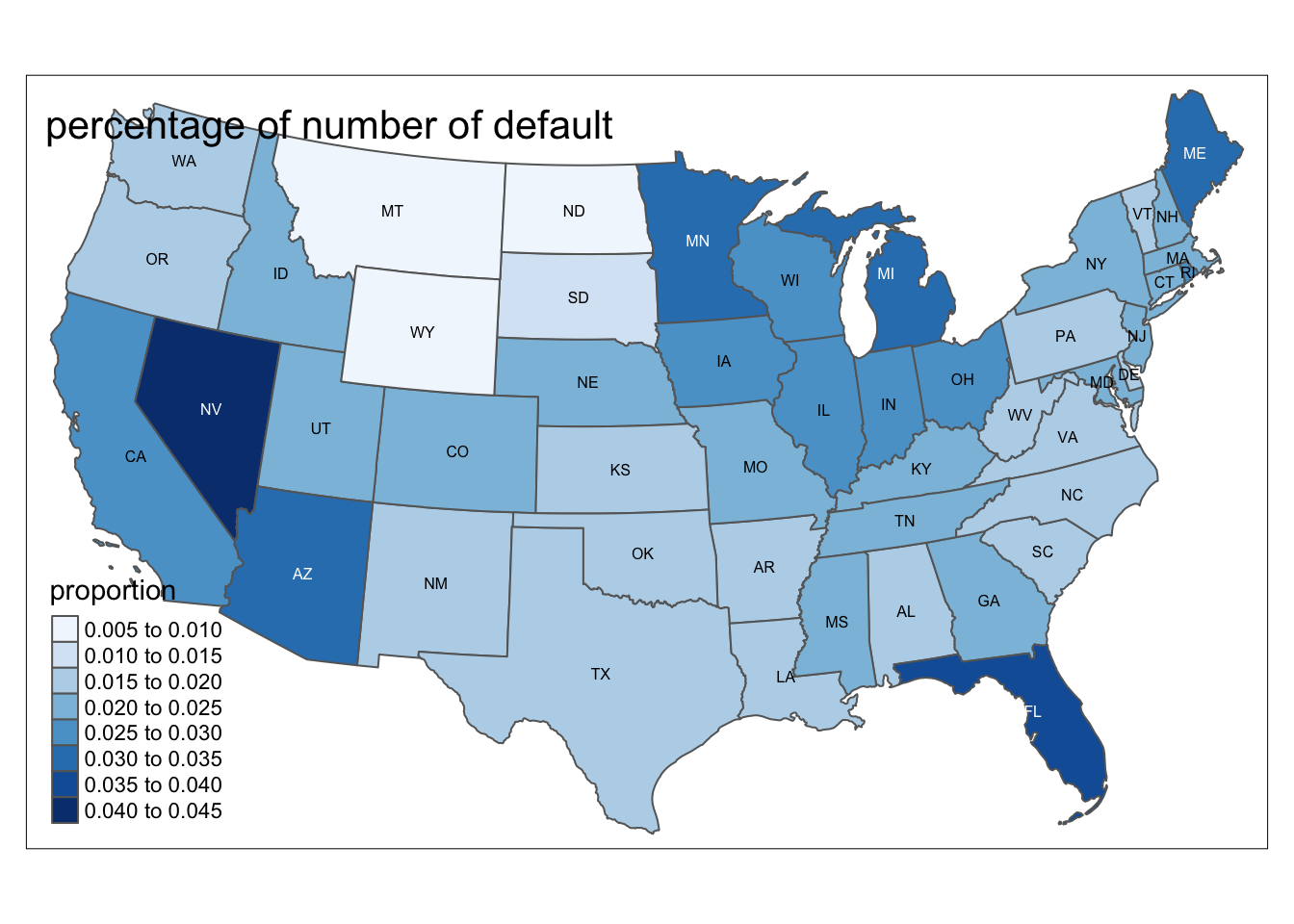
\[\\[0.2in]\]
This map shows the portion of number of default cases in each state in US. We can see from the map that west coast and Southeastern coast, including CA, NV and FL, has the highest proportion of default cases, which is around 2.5% to 4,5%. Then around Northeastern, including MN, MI, ME and OH, has the second highest proportion of default cases, which is around 2% to 3.5%. Northwestern, middle south and eastern coast has the lowest proportion of default cases, which is around 0.5% to 2%. However, we decided not to included state as an variable in our dataset since there will be 50 more dummy variables to be added. \[\\[0.1in]\]
After our EDA, we would like to have a feature selection to determine which variables to be kept in our dataset. We would like to use the leaps packages to specific variables to be included in our model. We would like to use the exhaustive method and have a maximum of 12 variables: \[\\[0.2in]\]
Modeldata <- mortgage_norm %>% select(default_time,orig_time, REtype_SF_orig_time,investor_orig_time, balance_orig_time,FICO_orig_time, LTV_orig_time, interest_rate_mean, hpi_orig_time,uer_mean,gdp_mean,age,SP)
leaps_fit <- leaps::regsubsets(default_time ~ ., data = Modeldata, method = 'exhaustive', nvmax = 12)
\[\\[0.2in]\]
As followed, we would like to visualize the result of the feature selection: \[\\[0.2in]\]
a <- as.tibble(summary(leaps_fit)$cp)
b <- as.tibble(summary(leaps_fit)$bic)
c <- as.tibble(summary(leaps_fit)$adjr2)
a$Number <- seq(1,12,1)
b$Number <- seq(1,12,1)
c$Number <- seq(1,12,1)
Performance <- a %>% left_join(b, by = 'Number') %>% left_join(c, by = 'Number')
names(Performance) = c('CP','Number','BIC','AdjustedR2')
ggplot(Performance, aes(y = BIC))  + geom_point(aes(x = factor(Number),size = AdjustedR2),color = 'steelblue4')+ geom_line(aes(x = Number),color = 'steelblue4')+theme_bw()+labs(x = 'Number of Variables', y = 'BIC',title = 'Compare BIC, Adjusted R Sqaure and Number of Variables')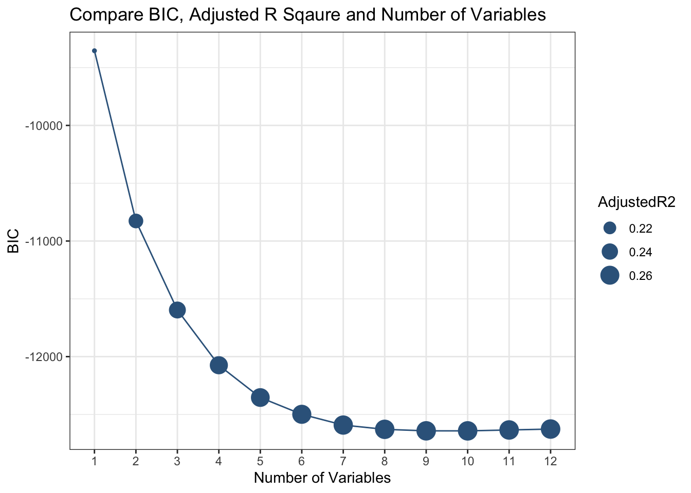
\[\\[0.2in]\]
As we can see from the chart here that as the number of variables increases, BIC decreases and Adjusted R square increases, which means that our performance of our model is getting better. With more than 9 variables, our model tends to have an adjusted R square of around 25%, which means that 25% of the variation in default or not can be explained by our explanatory variables. The model with 10 variables has lowest BIC(-12642.253) and relatively high adjusted R square(26.41291%) , therefore, we would like to choose the model with 10 variables. We would like to exclude original balance and original time in our model indicated by our feature selection result.
\[\\[0.2in]\]
Before making the model, we would like to separate our dataset into train and test dataset, we will choose choose a randomized 70% household for training data, and the rest for test data.(Code from https://www.statology.org/confusion-matrix-in-r/)
\[\\[0.2in]\]
data <- mortgage_norm
set.seed(1)
sample <- sample(c(TRUE, FALSE), nrow(data), replace=TRUE, prob=c(0.7,0.3))
train <- data[sample, ]
test <- data[!sample, ]
\[\\[0.2in]\]
Logistic:
\[\\[0.2in]\]
Logistic_Model <- glm(default_time ~ age  + REtype_SF_orig_time+
interest_rate_mean+gdp_mean+hpi_orig_time+uer_mean+investor_orig_time+FICO_orig_time+LTV_orig_time+age+SP, data = train, family = binomial)
Logistic_Model %>% broom::tidy() %>% knitr::kable()| term | estimate | std.error | statistic | p.value |
|---|---|---|---|---|
| (Intercept) | -2.6365954 | 0.3974081 | -6.634478 | 0.0000000 |
| age | -0.0320742 | 0.0039051 | -8.213473 | 0.0000000 |
| REtype_SF_orig_time | -0.0732574 | 0.0300077 | -2.441289 | 0.0146349 |
| interest_rate_mean | 0.0847245 | 0.0107629 | 7.871919 | 0.0000000 |
| gdp_mean | -0.9296961 | 0.0197045 | -47.181932 | 0.0000000 |
| hpi_orig_time | 0.0043628 | 0.0006793 | 6.422165 | 0.0000000 |
| uer_mean | 0.0498199 | 0.0207821 | 2.397251 | 0.0165186 |
| investor_orig_time | 0.3718477 | 0.0455207 | 8.168753 | 0.0000000 |
| FICO_orig_time | -0.0062101 | 0.0002497 | -24.872589 | 0.0000000 |
| LTV_orig_time | 0.0259683 | 0.0015637 | 16.607045 | 0.0000000 |
| SP | 0.0031322 | 0.0001995 | 15.701400 | 0.0000000 |
\[\\[0.2in]\]
As followed, we would like to use the Caret package to plot the importance of each variables in our model to determine their weights to predict default rate. \[\\[0.2in]\]
Imp <- varImp(Logistic_Model, scale = FALSE) %>% arrange(desc(Overall))
Imp %>% mutate(var = rownames(Imp)) %>% mutate(Variables = fct_reorder(var, Overall)) %>% ggplot(aes(y = Overall, x = Variables)) + geom_col(fill = 'steelblue4') + coord_flip()+ theme_bw()+labs(x = ' Variables', y = 'Importance',title = 'Variable Importance in Logistic Model')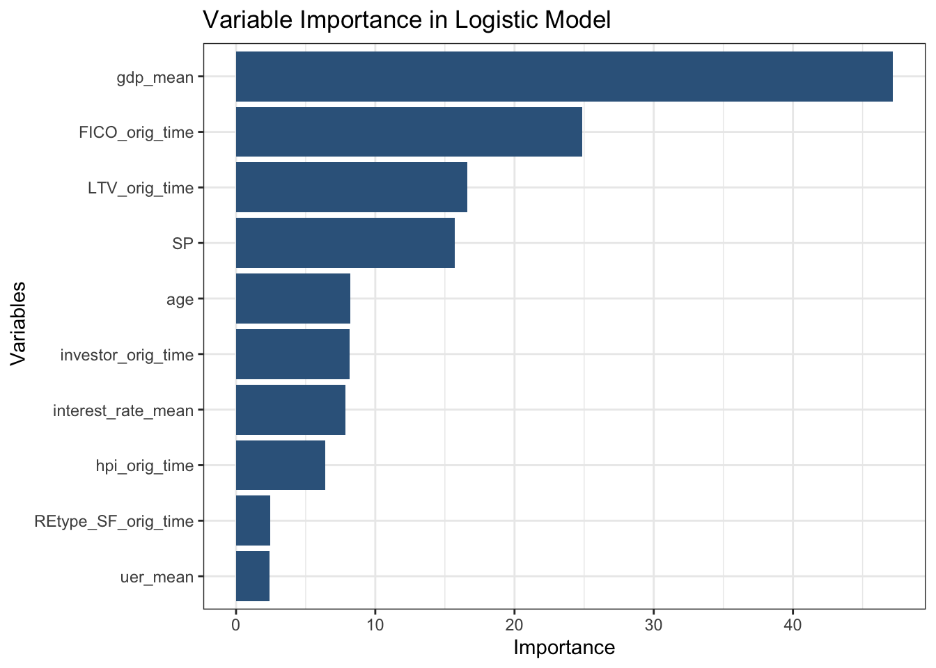
As we can see from the chart here, mean GDP growth and S&P stock index is the most outside economic variables to determine default rate in mortgage market. This is reasonable-as the economy of the country rises, more people have a good job and can afford to payoff the mortgage. Therefore, GDP growth is the dominant determinant when considering to give a mortgage or not. Meanwhile, FICO score and original loan to value are the second and third most important factor to be considered when making mortgages. This tells us that personal characteristics also plays an important roll when considering to give a mortgage or not. Therefore, when trying to measure the probability of default, banks should consider both outside economic data and inside personal information. Only by a comprehensive consideration can we better measure the credit risk inside the mortgage market. As followed, we would like to measure the overall performance of our model by adpating the model to our test data.
\[\\[0.2in]\]
Confusion Matrix For Logistic Model on Test Data:
\[\\[0.2in]\]
predicted <- predict(Logistic_Model, test, type="response")
optimal <- optimalCutoff(test$default_time, predicted)
b <- confusionMatrix(test$default_time, predicted)
TClass <- factor(c(0, 0, 1, 1))
PClass <- factor(c(0, 1, 0, 1))
Y      <- c(6615,1270, 1843 , 2746)
df <- data.frame(TClass, PClass, Y)
ggplot(data =  df, mapping = aes(x = TClass, y = PClass)) +
  geom_tile(aes(fill = Y), colour = "white") +
  geom_text(aes(label = sprintf("%1.0f", Y)), vjust = 1, color = 'white') +
  scale_fill_gradient(low = "skyblue", high = "steelblue3") +
  theme_bw() + theme(legend.position = "none")+ labs(title = 'Confusion Matrix For Logistic Model')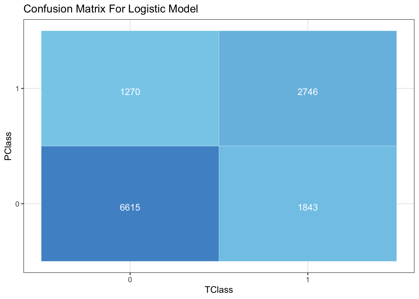
Shown by the confusion matrix, the model has a overall accuracy of about 75% on test data, with true positive of 2746 and true negative of 6615 out of about 12000 mortgages, which can be considered effective. As followed, we would like to measure it by ROC curve by ploting an ROC curve on test data.
\[\\[0.2in]\]
LinearData <- test %>% add_predictions(Logistic_Model, type = 'response')
roc(LinearData$default_time,LinearData$pred,plot = TRUE)
## Setting levels: control = 0, case = 1## Setting direction: controls < cases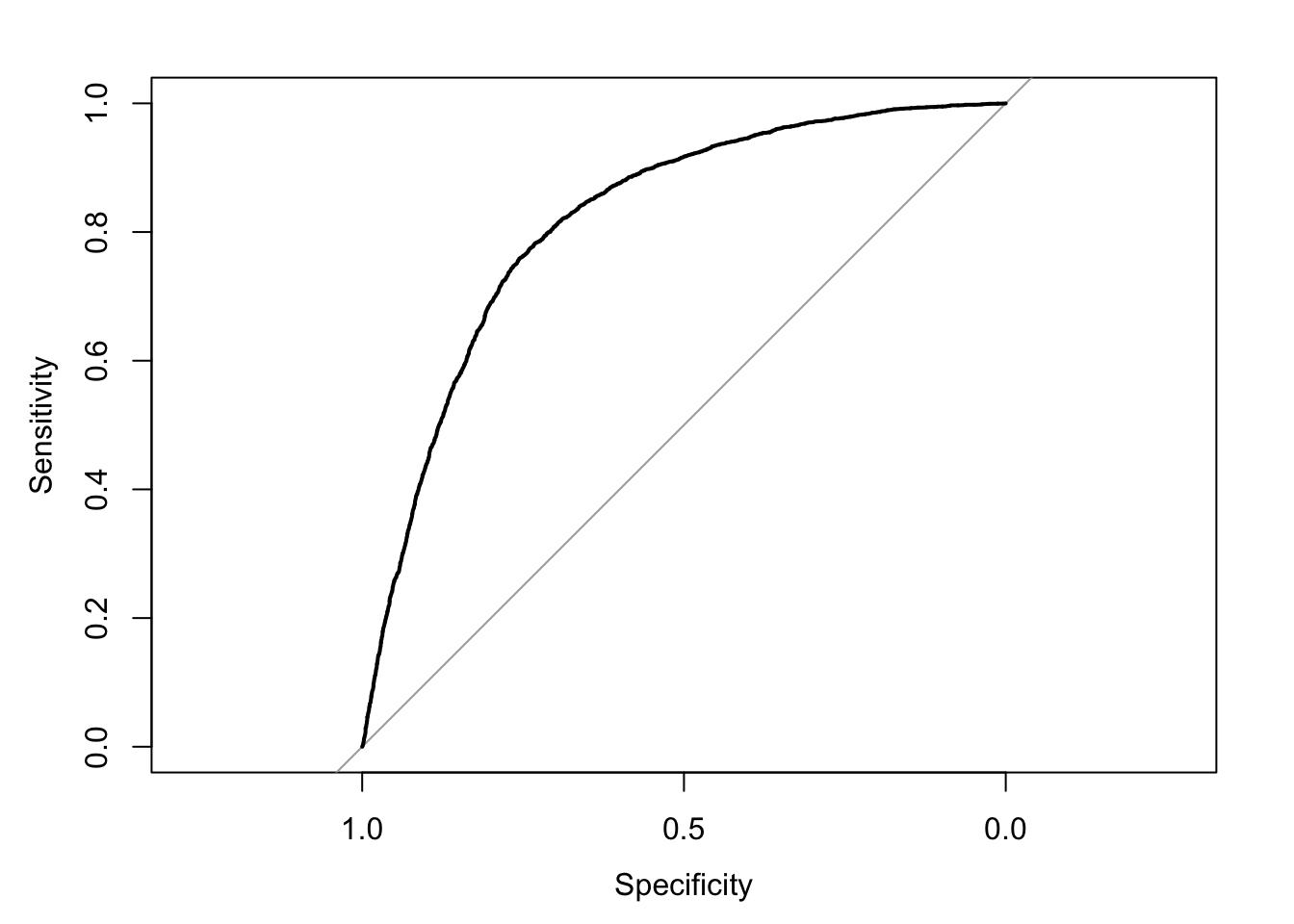
##
## Call:
## roc.default(response = LinearData$default_time, predictor = LinearData$pred,     plot = TRUE)
##
## Data: LinearData$pred in 7885 controls (LinearData$default_time 0) < 4589 cases (LinearData$default_time 1).
## Area under the curve: 0.8177
\[\\[0.2in]\]
We would like to use the pROC package. An ROC curve is one of the best way to measure the performance of model with output between 0 and 1, which corresponds to our default probability. In a ROC curve, an AUC of 0.5 is considered just guessing. As we can see here, our model has an AUC of 0.8163, which can be considered excellent. This is the end for our logistic model.
\[\\[0.2in]\]
Addtional Models
Before making our model, we read a few papers online and discovered that a lot of banks use models other logistic regression to measure the risk of default including K-Nearest Neighbor, Lasso Regression, Ada boosting, Neural Network, and RandomForest. Most papers considered RandomForest and Lasso as a better model to measure default rate compare to logistic regression. Therefore we would like to fit the variables given by leaps package in these models to see if they can do a better job.
\[\\[0.2in]\]
RandomForest:
\[\\[0.1in]\]
RandomForest model derives from the idea of decision tree model.
\[\\[0.2in]\]
Decision tree learning is one of the predictive modelling method used in data science and machine learning. It uses a decision tree (as a predictive model) to go from observations about an item (represented in the branches) to conclusions about the item’s target value (represented in the leaves). Classification tree models where the target variable can take a discrete set of values. In these tree structures, leaves represent class labels and branches represent conjunctions of features that lead to those class labels. Therefore, as the more data provided, more branches are created. In that case, the model is getting better in predicting target velue.
\[\\[0.2in]\]
However, one important issue with the decision tree model is overfitting. As the number of leaves increasing, the problem of overfitting rises as well, because we took the noise in the dataset into account also. Therefore, the idea of ranfomForest is created to avoid this problem. RandomForest bootstraps the training dataset to grow a decision tree in each subdataset with a number of randomly selected variables as its branches. Therefore, multiple instead of one decision tree are created to make the model. Each of these trees will give a final result on default or not. Then each result count as a vote on default or not, and the final probability of default is given by the portion of votes on defaults by all these trees. We start by training the model with train dataset.
\[\\[0.2in]\]
trainrf <- train %>% mutate(Default = as.factor(default_time))
testrf <- test %>% mutate(Default = as.factor(default_time))
rf <- randomForest(Default ~ age + REtype_SF_orig_time+
interest_rate_mean+gdp_mean+hpi_orig_time+uer_mean+investor_orig_time+FICO_orig_time+LTV_orig_time+age+SP, family = binomial, data = trainrf,importance=TRUE)
\[\\[0.2in]\]
As followed, I would like to examine the performance by plotting it into ROC curve on test dataset
\[\\[0.1in]\]
predicted <- as.tibble(predict(rf, testrf, type="vote"))[1]
colnames(predicted)[1] <- 'predict'
testrf <- testrf %>% mutate(pred = predicted$predict)
roc(testrf$default_time,testrf$pred,plot = TRUE)
## Setting levels: control = 0, case = 1## Setting direction: controls > cases
##
## Call:
## roc.default(response = testrf$default_time, predictor = testrf$pred,     plot = TRUE)
##
## Data: testrf$pred in 7885 controls (testrf$default_time 0) > 4589 cases (testrf$default_time 1).
## Area under the curve: 0.8432
\[\\[0.2in]\]
As we can see from the ROC curve, the randomForest model has a much higher AUC, which is about 0.85 compare to that of the logistic model(0.81). We believe that is because a logistic model can avoid overfitting. By growing a number of trees and give the probability of the mean value of independent votes, the noise in sub-dataset will not effect the overall predict result because of the central limit theorem. However, one disadvantage of random forest model is that it gives little detail explanation on the influence of each variables. What is more, we also do not know we the model comes to this result since the whole machine learning is invisible to us.Here, We use the Caret package again to have a glance of the importance of different variables in the model.
\[\\[0.2in]\]
importance(rf,type = 2)## MeanDecreaseGini
## age 653.8986
## REtype_SF_orig_time 263.7848
## interest_rate_mean 1952.1886
## gdp_mean 2658.9678
## hpi_orig_time 1461.1258
## uer_mean 1336.5263
## investor_orig_time 164.3199
## FICO_orig_time 2148.8718
## LTV_orig_time 1173.4905
## SP 1288.8551varImpPlot(rf)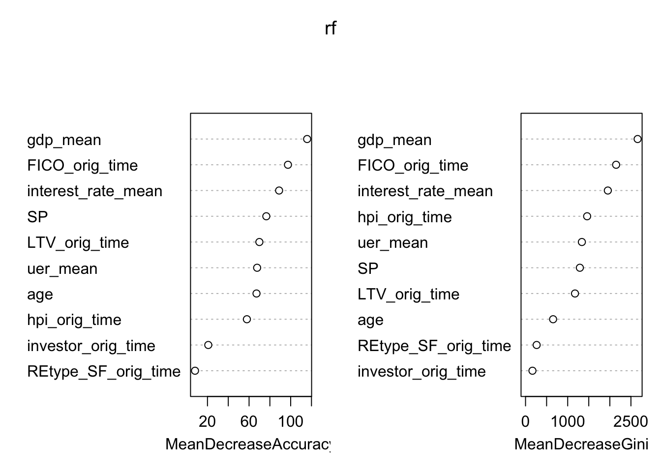
\[\\[0.2in]\]
Apparently, FICO score, GDP growth, and LTV is still the predominant factor to consider one’s default ability in this model. However, Compare to our logistic model, Unemployment Rate has is much more important in the Random Forest model. We still do not know the reason. However, we are sure that the ability of individual variable to predict target value is different in Logistic and Random Forest Model.
\[\\[0.2in]\]
Lasso Regression:
\[\\[0.2in]\]
This model is inspired by Stanford’s introduction to glmnet package written by Trevor Hastie, Junyang Qian, and Kenneth Tay.
lasso (least absolute shrinkage and selection operator; also Lasso or LASSO) is a regression analysis method that performs both variable selection and regularization in order to enhance the prediction accuracy and interpret-ability of the resulting statistical model.
\[\\[0.2in]\]
To start the Lasso Regession (with machine learning), we started by using similar partition idea in logistic regression:
\[\\[0.2in]\]
data_lasso <- mortgage_norm
set.seed(1)
sample <- sample(c(TRUE, FALSE), nrow(data), replace=TRUE, prob=c(0.7,0.3))
train.data <- data_lasso[sample, ]
test.data <- data_lasso[!sample, ]
\[\\[0.2in]\]
By applying R function glmnet() [glmnet package] for computing penalized logistic regression. The usage of variables are described as follow: x: matrix of predictor variables y: the response or outcome variable, which is a binary variable. *alpha: the elasticnet mixing parameter. Allowed values include: “1”: for lasso regression “0”: for ridge regression **a value between 0 and 1 for elastic net regression. *lamba: a numeric value defining the amount of shrinkage.
\[\\[0.2in]\]
x <- model.matrix(default_time ~ age  + REtype_SF_orig_time+
interest_rate_mean+gdp_mean+hpi_orig_time+uer_mean+investor_orig_time+FICO_orig_time+LTV_orig_time+age+SP, data = train.data)[,-1]

y <- ifelse(train.data$default_time == 1, 1, 0)
fit <- glmnet(x, y, family = "binomial")
x.test <- model.matrix(default_time ~ age + REtype_SF_orig_time+
interest_rate_mean+gdp_mean+hpi_orig_time+uer_mean+investor_orig_time+FICO_orig_time+LTV_orig_time+age+SP, test.data)[,-1]
set.seed(123)
cvfit <- cv.glmnet(x, y, family = "binomial", type.measure = "class")
plot(cvfit)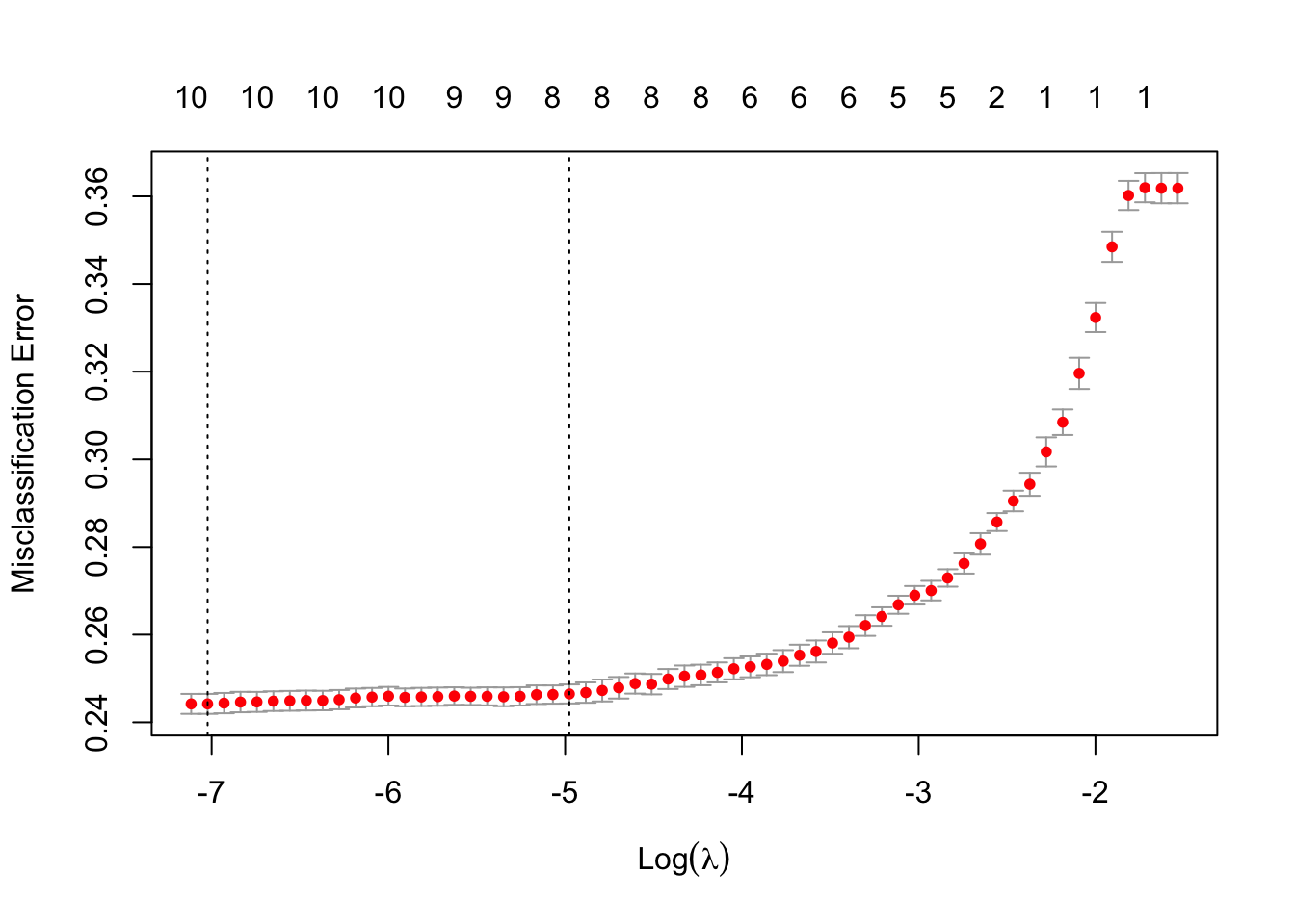
\[\\[0.2in]\]
\[\\[0.2in]\]
We started by working with similar methods in logistic regression, and we use glmnet package to plot the cvfit which enables us to see the optimal values of lambda. This lambda value will give the most accurate model.
\[\\[0.2in]\]
We received two different lambdas. lambda.min gives a model with the smallest number of predictors that also gives a good accuracy, while lambda.1se gives the simplest model but also lies within one standard error of the optimal value of lambda. This value is called lambda.1se. We can see the coefficient in the following code
\[\\[0.2in]\]
cvfit$lambda.min## [1] 0.0008913206cvfit$lambda.1se## [1] 0.006901172\[\\[0.2in]\]
coef(cvfit, cvfit$lambda.1se)## 11 x 1 sparse Matrix of class "dgCMatrix"
## s1
## (Intercept) -1.860096870
## age -0.014434603
## REtype_SF_orig_time .
## interest_rate_mean 0.079379688
## gdp_mean -0.875595002
## hpi_orig_time 0.005392535
## uer_mean .
## investor_orig_time 0.226750768
## FICO_orig_time -0.005145818
## LTV_orig_time 0.020511852
## SP 0.002277904coef(cvfit, cvfit$lambda.min)## 11 x 1 sparse Matrix of class "dgCMatrix"
## s1
## (Intercept) -2.430491815
## age -0.029035220
## REtype_SF_orig_time -0.060951181
## interest_rate_mean 0.083178440
## gdp_mean -0.926336403
## hpi_orig_time 0.004557043
## uer_mean 0.034897747
## investor_orig_time 0.353332819
## FICO_orig_time -0.006062420
## LTV_orig_time 0.025218146
## SP 0.002970744\[\\[0.2in]\]
As we can see from above, in lambda.1se, variables uer_mean and REtype_SF_orig_time are penalized to 0, which means that these two variables are kicked out by lasso’s nature of penalization. In this model, we will use lambda.1se to fit the model.
\[\\[0.2in]\]
Then, we plot the ROC curve:
cfit <- cv.glmnet(x, y, family = "binomial", type.measure = "auc",
                  keep = TRUE)
rocs <- roc.glmnet(cfit$fit.preval, newy = y)

best <- cvfit$index["min",]
plot(rocs[[best]], type = "l")
invisible(sapply(rocs, lines, col="grey"))
lines(rocs[[best]], lwd = 2,col = "blue")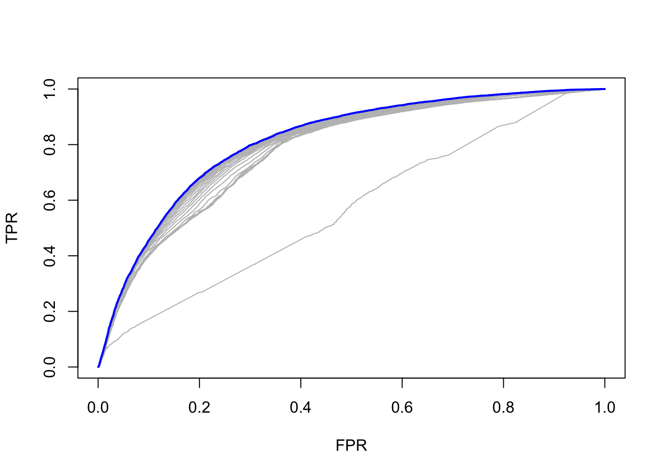
\[\\[0.2in]\]
Finally, we fit the model by using lambda 1se and check the accuracy of the model:
\[\\[0.2in]\]
# Final model with lambda.1se
lasso.model <- glmnet(x, y, alpha = 1, family = "binomial",
                      lambda = cvfit$lambda.1se)
# Make prediction on test data
x.test <- model.matrix(default_time ~ age  + REtype_SF_orig_time+
interest_rate_mean+gdp_mean+hpi_orig_time+uer_mean+investor_orig_time+FICO_orig_time+LTV_orig_time+age+SP,   test.data)[,-1]
probabilities <- lasso.model %>% predict(newx = x.test)
predicted.classes <- ifelse(probabilities > 0.5, 1, 0)
# Model accuracy rate
observed.classes <- test.data$default_time
mean(predicted.classes == observed.classes)
## [1] 0.7138849\[\\[0.2in]\]
Overall, the Lasso method kicked out two variables because of penalization, and overall accuracy was 0.71, which is fairly a strong model.
Conclusion
\[\\[0.2in]\]
Overall, after our analysis and modeling, we believe that mortgage issuer should adopt different kinds of information to different models to measure the credit risk of specific mortgages.
\[\\[0.2in]\]
Three modeling methods all agree that GDP, FICO Score, and Loan to Value Ratio will play important roles in people’s behaviors of whether paying or not paying back their mortgages. As issuers and financial analysts, the aggregate change of these variables should be closely examine. Moreover, different models tend to select different variables playing a minor role in the story — logistic regression and lasso regression manifest that whether an individual is in single family or not does not have significant correlation the default probability for lenders, and unemployment rate does not as well. This counters our intuition, but it is understandable – while unemployed and single-family people are not able to pay back, their willingness to apply mortgages are low. Random Forest gives us the result that whether one is with investor is minor in the correlation as well. SO, it is important to combine different models.
\[\\[0.2in]\]
By applying different models, different variables’ importance are re-evaluated, and we also realized that forecasting modeling is somehow subjective, which make me believe that using different models to forecast are the right thing to do.